If two traits (A and b) are associated with another trait C at the same time, we can test whether trait C affects trait B through trait a or vice versa through intermediary analysis. This paper will take you to a simple intermediary analysis.
Theoretical knowledge
principle
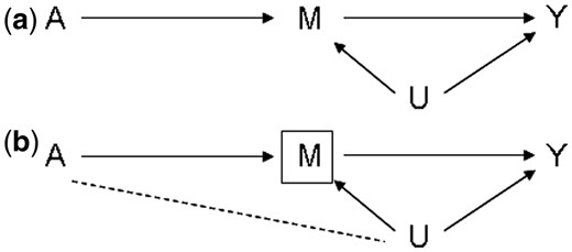
The importance of intermediary analysis in epidemiological research is to reveal the impact of exposure on results. Mediation analysis is usually used to evaluate the extent to which the impact of exposure is explained, or when there is no assumed mediation variable (also known as intermediate variable), in this way, the total impact of exposure on results can be defined, The effects of exposure by a given set of mediators (indirect effects) and the effects of exposure that cannot be explained by these same mediators (direct effects)

Generally, the part that can be explained by intermediary variables is indirect effect, and the part that cannot be explained by these intermediary variables is direct effect. People expect that the total effect can be decomposed into direct effect and indirect effect, that is, assuming that the exposure factors have 15% risk, in which the risk of direct effect is 10%, the risk of indirect effect is 5%, in other words, One third of the total effects can be explained by intermediary variables, and the other two-thirds of the total effects can be explained by other ways
[scode type="yellow"]
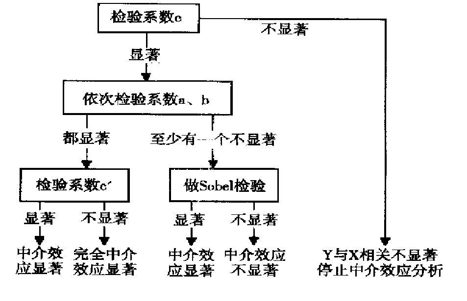
Generally, the test of intermediary effect is considered only when the independent variable has an impact on the dependent variable (with a total effect). However, the fact that the independent variable has no impact on the dependent variable does not mean that there is no intermediate variable, but the impact at this time is called indirect effect. Intermediary effects are indirect effects, but indirect effects are not necessarily intermediary effects. In real life, the effect direction between independent variable and intermediate variable, intermediate variable and dependent variable is opposite, so that the total effect is 0. This situation is called effect masking, that is, generalized intermediate effect.
[/scode]
There are many reviews on intermediary analysis. Here are two articles, one in Chinese and one in English, for reference:
Estimation of mediating effect
The calculation of mediation effect is particularly simple, which is briefly described as follows:
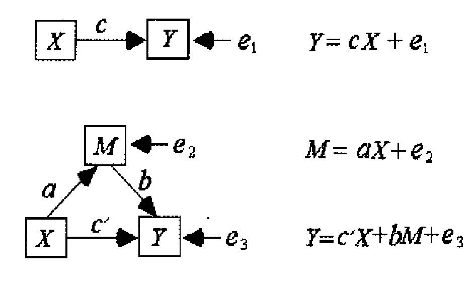
- First, the total effect is estimated. The total effect should be the overall effect of the independent variable on the dependent variable, generally:
- Then estimate the correlation between independent variables and intermediate variables:
- Finally, estimate the direct effect, that is, the effect of the independent variable corrected by the intermediary variable on the dependent variable, also known as the direct effect:
- Now, the total effect is \ (c \), the direct effect is \ (c '\), the intermediary effect is \ (c - c' \), and the proportion of intermediary effect is \ (\ frac {c - c'} {c} \)
Test of mediating effect
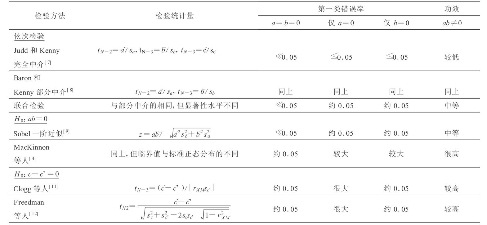
Compared with the estimation of mediation effect, the test of mediation effect is slightly more complex, and Sobel test is commonly used
The parameters in the following inspection methods are from the following figure:


Practice of intermediary analysis
After understanding the principle of intermediary analysis and the statistical method of test, an example is given to illustrate the process of intermediary analysis.
Design simulation data
Using the data of R's own iris for simulation research, here we define sepal length sepal Length is an independent variable, named X, which defines its attraction to bees as an intermediary variable and named M. We define a dependent variable. We assume that its meaning is the possibility of being finally collected by bees, named Y. in order to create some noise and intermediary effects, we define the following relationship between these three variables:
In this way, our expected mediating effect is 12.25%, and then we will test it
Create simulation data
df=iris
set.seed(12334)

colnames(df)[1] = "X"

df$e1 = runif(nrow(df), min = min(df$X), max = max(df$X))
df$M = df$X * 0.35 + df$e1 * 0.65

df$e2 = runif(nrow(df), min = min(df$M), max = max(df$M))
df$Y = df$M * 0.35 + df$e2 * 0.65
Test total effect
The test equation is:
The inspection code is:
fit_total = lm(Y ~ X, df)
summary(fit_total)
The output is as follows:
Call:
lm(formula = Y ~ X, data = df)

Residuals:
     Min       1Q   Median       3Q      Max
-1.15930 -0.45815 -0.01242  0.44662  1.20905

Coefficients:
            Estimate Std. Error t value Pr(>|t|)
(Intercept)  5.29106    0.32791  16.136   <2e-16 ***
X            0.12984    0.05557   2.337   0.0208 *
---
Signif. codes:  0 '***' 0.001 '**' 0.01 '*' 0.05 '.' 0.1 ' ' 1

Residual standard error: 0.5616 on 148 degrees of freedom
Multiple R-squared:  0.03558,	Adjusted R-squared:  0.02907
F-statistic:  5.46 on 1 and 148 DF,  p-value: 0.02079
It can be seen that the total effect is 0.12984, close to our expectation of 12.25%, and the p value is 0.0208. The first step test is significant, and then proceed to the following steps
Test the effect of dependent variables on intermediate variables
The test equation is:
The inspection code is:
fit_mediator = lm(M ~ X, df)
summary(fit_mediator)
The output is as follows:
Call:
lm(formula = M ~ X, data = df)

Residuals:
    Min      1Q  Median      3Q     Max
-1.2494 -0.5082  0.0123  0.5483  1.0799

Coefficients:
            Estimate Std. Error t value Pr(>|t|)
(Intercept)  4.32300    0.37901  11.406  < 2e-16 ***
X            0.30429    0.06422   4.738 5.02e-06 ***
---
Signif. codes:  0 '***' 0.001 '**' 0.01 '*' 0.05 '.' 0.1 ' ' 1

Residual standard error: 0.6492 on 148 degrees of freedom
Multiple R-squared:  0.1317,	Adjusted R-squared:  0.1258
F-statistic: 22.45 on 1 and 148 DF,  p-value: 5.019e-06
It can be seen that the effect of the intermediary variable on the dependent variable is 0.30429, close to our expectation of 35%, and the p value is 5.019e-06. The second test is also significant, and then proceed to the following steps
Test direct effect
The test equation is:
The inspection code is:
fit_direct=lm(Y ~ X + M, df)
summary(fit_direct)
The output is as follows:
Call:
lm(formula = Y ~ X + M, data = df)

Residuals:
     Min       1Q   Median       3Q      Max
-0.90734 -0.46316  0.00764  0.39751  0.87026

Coefficients:
            Estimate Std. Error t value Pr(>|t|)
(Intercept)  3.68314    0.40721   9.045 8.17e-16 ***
X            0.01667    0.05402   0.309    0.758
M            0.37194    0.06443   5.773 4.46e-08 ***
---
Signif. codes:  0 '***' 0.001 '**' 0.01 '*' 0.05 '.' 0.1 ' ' 1

Residual standard error: 0.5088 on 147 degrees of freedom
Multiple R-squared:  0.2138,	Adjusted R-squared:  0.2031
F-statistic: 19.99 on 2 and 147 DF,  p-value: 2.092e-08
It can be seen that the direct effect is 0.016, which is very weak, and the p value is 0.758, which is not significant, while the effect value of the intermediary variable on the dependent variable is 0.37194, which is close to our expectation of 35%, and the p value is 4.46e-08. This result shows that after the correction of the intermediary variable, the influence of the independent variable on the dependent variable is not significant, This situation is called complete mediation
sobel test
If both coefficient a and coefficient b are not significant, the significance of the mediating effect is calculated by the following formula. This method was proposed by Sobel, so it is called Sobel test:
Where \ (\ hat{a} \) is the effect of the independent variable on the intermediate variable, \ (\ hat{b} \) is the effect of the intermediate variable on the dependent variable after correction with the intermediate variable, \ (s_a \) and \ (s_b \) are the standard errors of \ (\ hat{a} \) and \ (\ hat{b} \) respectively. In the above results, it refers to the column Std. Error. The operation in R is as follows:
a = coefficients(fit_mediator)["X"]
s_a = summary(fit_mediator)$coefficients["X", "Std. Error"]
b = coefficients(fit_mediator)["M"]
s_b = summary(fit_direct)$coefficients["M", "Std. Error"]
SE = sqrt(a^2 * s_b^2 + b^2 * s_a^2)
# The degree of freedom is n-k-1, K is the number of explanatory variables, here it is 2, so df = 147
t_statistic = a * b / SE
p = 2 * pt(
	abs(t_statistic),
	df = df.residual(fit_mediator),
	lower.tail = FALSE
)
summary
In the above process, the overall effect of the independent variable on the dependent variable is 0.12984, and the influence coefficient of the independent variable on the intermediate variable and the influence coefficient of the intermediate variable on the dependent variable are close to our simulated 0.35. After correcting the influence of the intermediate variable, the influence (direct effect) of the independent variable on the dependent variable becomes very small (0.01667) and insignificant. Therefore, We can say that the influence of independent variables on dependent variables is completely through intermediary variables, which is called complete intermediary effect
Since the total effect is 0.12984 and the direct effect is 0.01667, the intermediary effect is 0.12984 - 0.01667 = 0.11317, accounting for 87.16%
Simplify operations with R packages
The above operation is a little cumbersome. Is there an R package that encapsulates this process? Of course, that is mediation:
install.packages("mediation")
library(mediation)

results = mediate(
	model.m  = fit_mediator,
	model.y  = fit_direct,
	treat    = "X",
	mediator = "M",
	boot     = TRUE
)
summary(results)
The results are as follows:
Causal Mediation Analysis

Nonparametric Bootstrap Confidence Intervals with the Percentile Method

               Estimate 95% CI Lower 95% CI Upper p-value
ACME             0.1132       0.0575         0.17  <2e-16 ***
ADE              0.0167      -0.0904         0.12   0.752
Total Effect     0.1298       0.0152         0.24   0.018 *
Prop. Mediated   0.8716       0.3796         3.68   0.018 *
---
Signif. codes:  0 '***' 0.001 '**' 0.01 '*' 0.05 '.' 0.1 ' ' 1

Sample Size Used: 150

Simulations: 1000
Here, ACME in the result represents the average mediation effect, which is equal to \ (\ hat{a}*\hat{b} \), ADE represents the direct effect, Total Effect is the Total Effect, and prop Mediated is the proportion of mediated effect
Generally, the product of the effect \ (\ beta_1 \) of the independent variable on the intermediary variable and the effect \ (\ beta_2 \) of the intermediary variable on the dependent variable is regarded as the average intermediary effect
Research using intermediary analysis
The following studies used mediation analysis
| data type | URL | Mediation method | explain |
|---|---|---|---|
| eQTL-meQTL | nature communications | Sobel | For each Co located data pair, the correlation analysis is carried out again and the mediation effect is tested |
| eQTL-pQTL | nature | mendelian randomization | Genetic variation as instrumental variable, plasma protein as exposure (i.e. pQTL), and disease as outcome |
| pQTL-eQTL | nature communications | mendelian randomization | The independent site (0.1) of GWAS was used as the instrumental variable, CHD as the outcome, and protein as the exposure (pQTL). The significance of multiple independent sites and individual sites was calculated by multipoint MR and wald test respectively. The tool was MRbase |