catalogue
1.AHP (analytic hierarchy process)
2.TOPSIS method (good and bad solution distance method)
2, Interpolation and fitting model
2. Fitting algorithm (cftool toolbox)
1, Evaluation model
1.AHP (analytic hierarchy process)
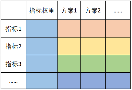
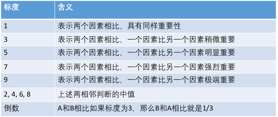
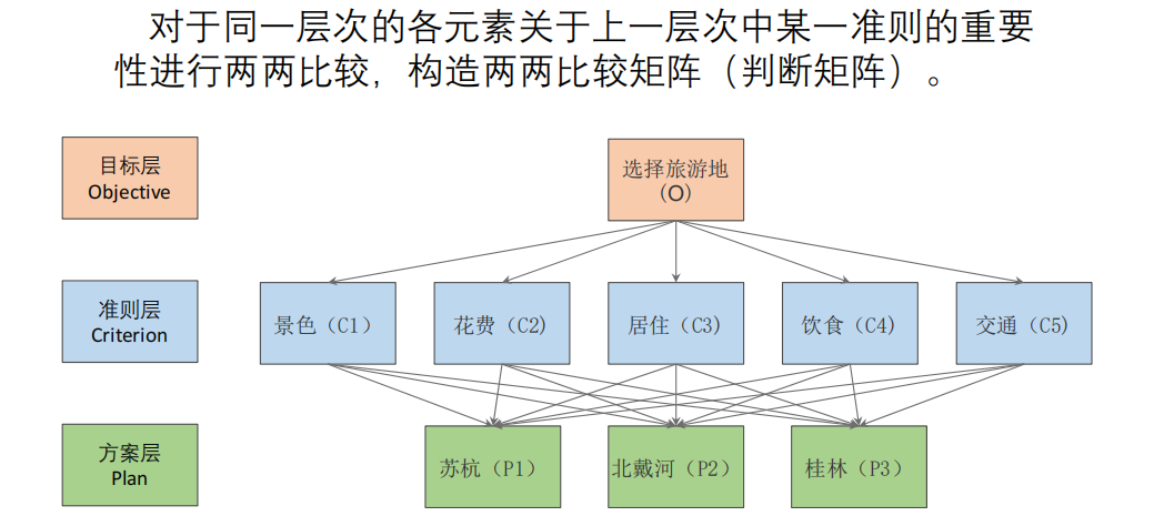
The most basic evaluation model solves evaluation problems through scoring (pairwise comparison and weight calculation).
Matlab code:
disp('Please enter the judgment matrix A')
A=input('A=');
[n,n] = size(A);

% Method 1: calculate the weight by arithmetic average method
Sum_A = sum(A);
SUM_A = repmat(Sum_A,n,1);
Stand_A = A ./ SUM_A;
disp('The result of weight calculation by arithmetic average method is:');
disp(sum(Stand_A,2)./n)

% Method 2: calculate the weight by geometric average method
Prduct_A = prod(A,2);
Prduct_n_A = Prduct_A .^ (1/n);
disp('The weight obtained by geometric average method is:');
disp(Prduct_n_A ./ sum(Prduct_n_A))

% Method 3: calculate the weight by eigenvalue method
[V,D] = eig(A);
Max_eig = max(max(D));
[r,c]=find(D == Max_eig , 1);
disp('The result of weight calculation by eigenvalue method is:');
disp( V(:,c) ./ sum(V(:,c)) )

% Calculate consistency ratio CR
CI = (Max_eig - n) / (n-1);
RI=[0 0.0001 0.52 0.89 1.12 1.26 1.36 1.41 1.46 1.49 1.52 1.54 1.56 1.58 1.59];
CR=CI/RI(n);
disp('Consistency index CI=');disp(CI);
disp('Consistency ratio CR=');disp(CR);

if CR<0.10
    disp('because CR<0.10,So the judgment matrix A The consistency of is acceptable!');
else
    disp('be careful: CR >= 0.10,Therefore, the judgment matrix A Modification required!');
end
2.TOPSIS method (good and bad solution distance method)
A commonly used comprehensive evaluation method, which can make full use of the information of the original data and reflect the gap between the evaluation schemes.
Improvement: Topsis method with weight (AHP or entropy weight method)
Matlab code:
load data_water_quality.mat
% Index forward
[n,m] = size(X);
disp(['share' num2str(n) 'Evaluation objects, ' num2str(m) 'Evaluation index'])
Judge = input(['this' num2str(m) 'Whether the indicators need to be processed forward or not, please enter 1 if necessary, and 0 is not required: ']);
if Judge == 1
Position = input('Please enter the column of the indicator that needs to be processed forward. For example, if the second, third and sixth columns need to be processed, you need to enter[2,3,6]: '); %[2,3,4]
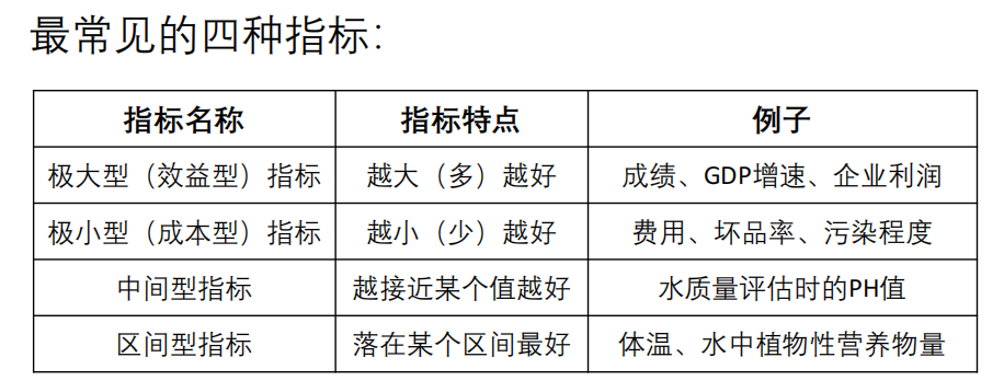
disp('Please enter the indicator type of these columns to be processed (1: very small, 2: intermediate, 3: interval) ')
Type = input('For example, if column 2 is very small, column 3 is interval type, and column 6 is intermediate type, enter[1,3,2]: '); %[2,1,3]
for i = 1 : size(Position,2)
X(:,Position(i)) = Positivization(X(:,Position(i)),Type(i),Position(i));
end
disp('Forward matrix X = ')
disp(X)
end
% Matrix standardization
Z = X ./ repmat(sum(X.*X) .^ 0.5, n, 1);
disp('Standardized matrix Z = ')
disp(Z)
% Need to add weight
disp("Please enter whether to increase the weight vector. You need to enter 1 instead of 0")
Judge = input('Please enter whether to increase the weight: ');
if Judge == 1
Judge = input('To determine the weight using entropy weight method, please enter 1, otherwise enter 0: ');
if Judge == 1
if sum(sum(Z<0)) >0
disp('Originally standardized Z There are negative numbers in the matrix, so you need to X Re standardization')
for i = 1:n
for j = 1:m
Z(i,j) = [X(i,j) - min(X(:,j))] / [max(X(:,j)) - min(X(:,j))];
end
end
disp('X Standardization matrix obtained by re standardization Z by: ')
disp(Z)
end
weight = Entropy_Method(Z);
disp('The weight determined by entropy weight method is:')
disp(weight)
else
disp(['If you have three indicators, you need to enter three weights, for example, they are 0.25,0.25,0.5, Then you need to enter[0.25,0.25,0.5]']);
weight = input(['You need to enter' num2str(m) 'Weights.' 'Please enter this as a line vector' num2str(m) 'Weights: ']);
OK = 0;
while OK == 0
if abs(sum(weight) -1)<0.000001 && size(weight,1) == 1 && size(weight,2) == m
OK =1;
else
weight = input('Your input is wrong, please re-enter the weight line vector: ');
end
end
end
else
weight = ones(1,m) ./ m ; %If you do not need to add weights, the default weights are the same, that is, they are all 1/m
end
% Calculate the distance from the maximum value and the minimum value, and calculate the score
D_P = sum([(Z - repmat(max(Z),n,1)) .^ 2 ] .* repmat(weight,n,1) ,2) .^ 0.5;
D_N = sum([(Z - repmat(min(Z),n,1)) .^ 2 ] .* repmat(weight,n,1) ,2) .^ 0.5;
S = D_N ./ (D_P+D_N);
disp('The final score is:')
stand_S = S / sum(S)
[sorted_S,index] = sort(stand_S ,'descend')2, Interpolation and fitting model
1. Interpolation algorithm
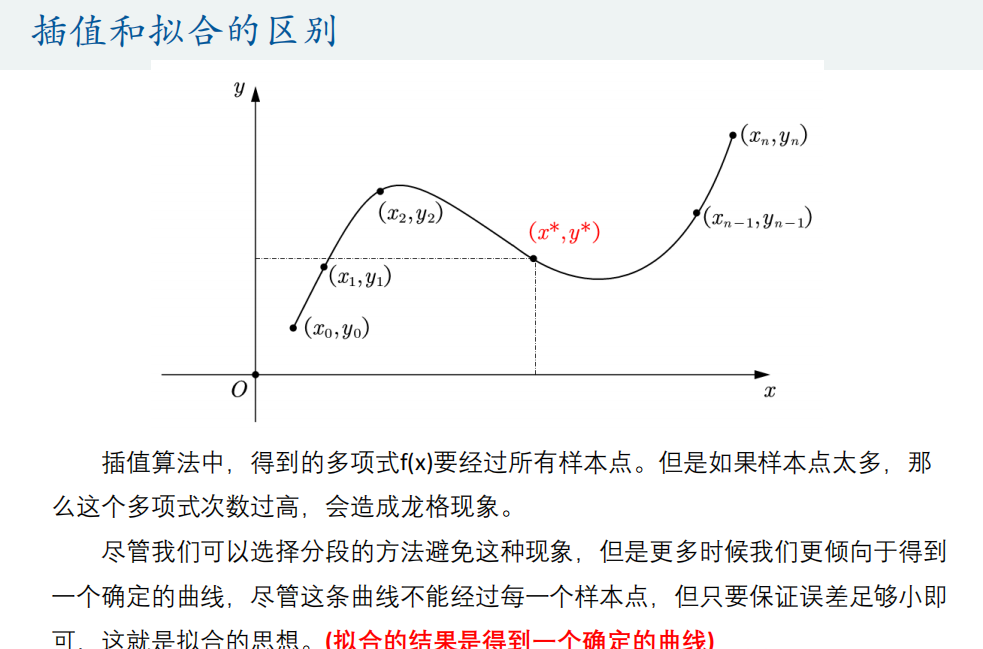
In mathematical modeling, it is often necessary to process and analyze the data and model according to the known function points, and sometimes the existing data is very few, which is not enough to support the analysis. At this time, some mathematical methods need to be used to "simulate" some new but reliable values to meet the needs, which is the role of interpolation.
Piecewise cubic Hermite interpolation & cubic spline interpolation
Matlab code:
% If you want to draw multiple figures in the same script file, you need to number each figure, otherwise only the last figure will be displayed

% plot Function usage:
% plot(x1,y1,x2,y2)
% Line mode: - Solid line :Point line -. Imaginary point line - - Zigzag line
% Point mode: . Dot  +plus  * asterisk  x x shape  o Small circle
% Color: y Yellow; r Red; g Green; b Blue; w White; k Black; m Purple; c young
x = -pi:pi;
y = sin(x);
new_x = -pi:0.1:pi;

% Piecewise cubic Hermite interpolation
p1 = pchip(x,y,new_x);

% Cubic spline interpolation
p2 = spline(x,y,new_x);

plot(x,y,'o',new_x,p1,'r-',new_x,p2,'b-')
legend('Sample point','Piecewise cubic Hermite interpolation','Cubic spline interpolation','Location','SouthEast') 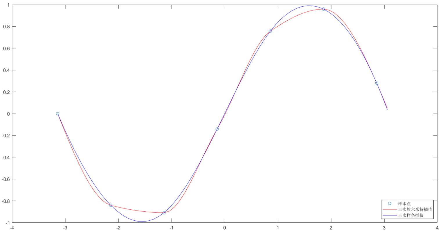
Conclusion: the curve generated by cubic spline interpolation is smoother. In actual modeling, because we do not know the data generation process, both interpolation methods can be used.
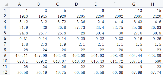
An example of Excel data interpolation
Matlab code:
%% Interpolation prediction of water body evaluation index in the middle week

load Z.mat
x=Z(1,:);
[n,m]=size(Z);

% be careful Matlab String cannot be saved in the array of. If you want to generate string array, you need to use cell array and curly braces{}Definitions and references
ylab={'Number of weeks','rotifer','Dissolved oxygen','COD','water temperature','PH value','salinity','transparency','Total alkalinity','Chloride ion','transparency','Biomass'};
disp(['share' num2str(n-1) 'Two indicators should be interpolated.'])

P=zeros(11,15);

for i=2:n
    y=Z(i,:);
    new_x=1:15;
    p1=pchip(x,y,new_x);
    subplot(4,3,i-1);
    plot(x,y,'ro',new_x,p1,'-');
    axis([0 15,-inf,inf])
    %  xlabel('week')
    ylabel(ylab{i})
    P(i-1,:)=p1;
end

legend('raw data','Cubic Hermite interpolation data','Location','SouthEast')

%hold P Add last week to the first line of
P = [1:15; P] 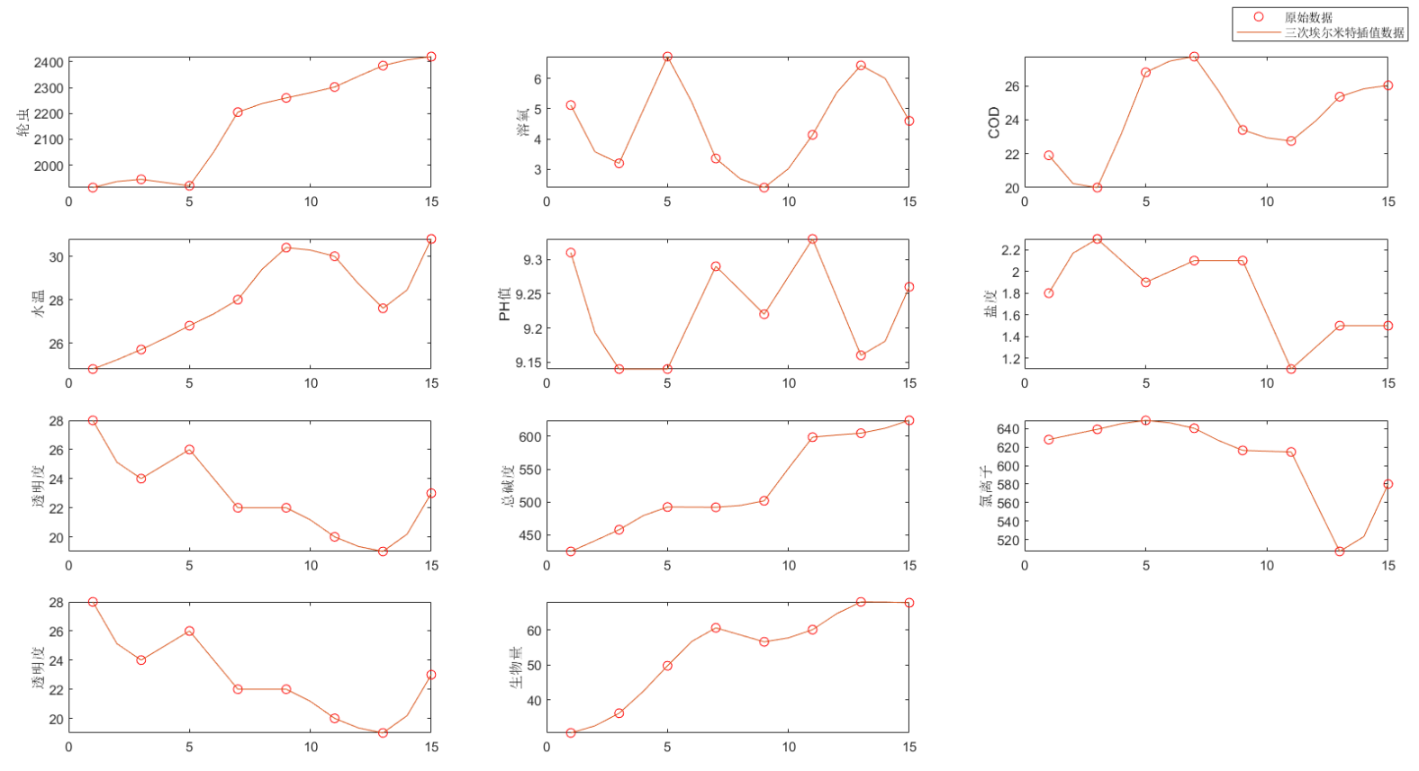
2. Fitting algorithm (cftool toolbox)
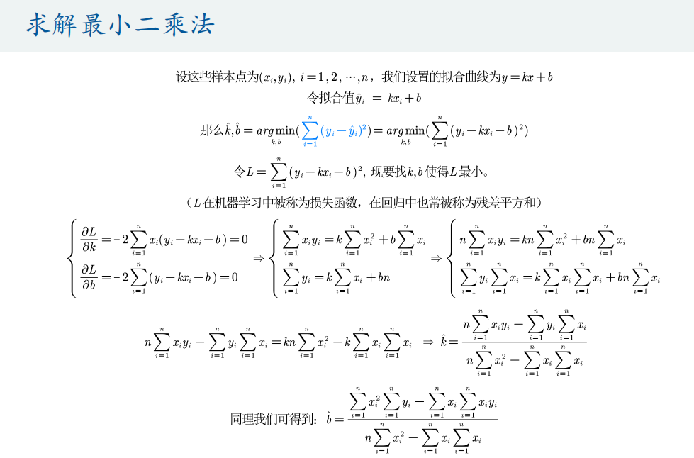
Different from the interpolation problem, the curve does not necessarily pass through a given point in the fitting problem. The goal of the fitting problem is to find a function (curve) so that the curve is closest to all data points under a certain criterion, that is, the curve fitting is the best (minimizing the loss function).
Matlab code:
load data1
plot(x,y,'o')
xlabel('x Value of')
ylabel('y Value of')
n = size(x,1);
k = (n*sum(x.*y)-sum(x)*sum(y))/(n*sum(x.*x)-sum(x)*sum(x))
b = (sum(x.*x)*sum(y)-sum(x)*sum(x.*y))/(n*sum(x.*x)-sum(x)*sum(x))
% Continue drawing on the previous figure
hold on
% display grid lines
grid on
f=@(x) k*x+b;
fplot(f,[2.5,7]);
legend('sample data ','Fitting function','location','SouthEast')
% y Fitting value of
y_hat = k*x+b;
% Regression sum of squares
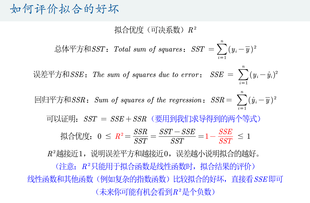
SSR = sum((y_hat-mean(y)).^2)
% Sum of squares of errors
SSE = sum((y_hat-y).^2)
% Total sum of squares
SST = sum((y-mean(y)).^2)
% Goodness of fit
R_2 = SSR / SST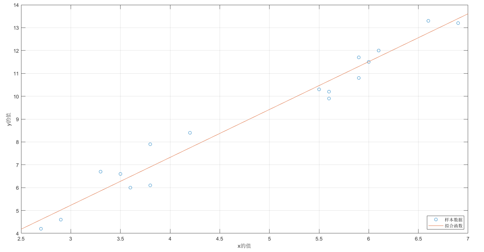
Powerful curve fitting toolbox: cftool
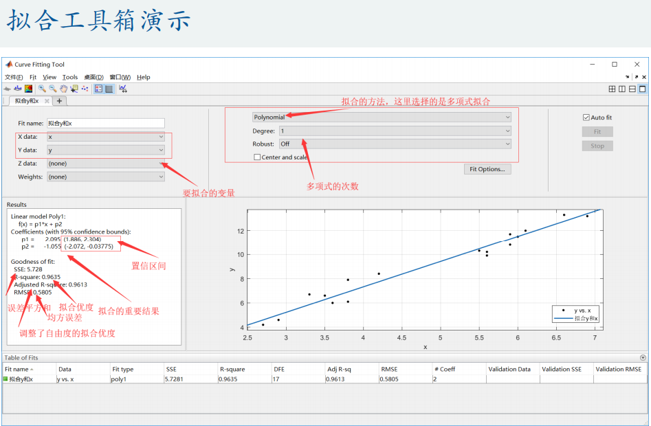
Pay attention to adjusting the starting point of Fit Options parameters!
(export image can be adjusted to high resolution in rendering settings)
Matlab code:
x = rand(30,1) * 10;
y = 3 * exp(0.5*x) -5 + normrnd(0,1,30,1);
% cftool
Content original author: mathematical modeling Qingfeng
Learning purpose, for reference only.