Ex3_ Machine learning_ Wu Enda's course assignment (Python): multi class classification & Neural Networks

instructions:

This article is about Mr. Wu Enda's learning notes of the machine learning course on Coursera.

• The first part of this paper first introduces the knowledge review and key notes of the corresponding week of the course, as well as the introduction of the code implementation library.
• The second part of this paper includes the implementation details of user-defined functions in the code implementation part.
• The third part of this paper is the specific code implementation corresponding to the course practice topic.

0. Pre-condition

This section includes some introductions of libraries.

# This file includes self-created functions used in exercise 3
import numpy as np
import matplotlib.pyplot as plt
import scipy.optimize as opt
from scipy.io import loadmat

00. Self-created Functions

This section includes self-created functions.

• loadData(path): read mat data

  # Load data from the given file
  def loadData(path):
      df = loadmat(path)
      X = df['X']
      y = df['y']
      return X, y
  

• Load weight (path): used for pre propagation algorithm to read the weight data of each layer of neural network

  # Load weight data from the given file
  def loadWeight(path):
      df = loadmat(path)
      return df['Theta1'], df['Theta2']
  

• plotOneImage(X, y): read and process the compressed gray image data and visualize it

  # Randomly pick a training example and visualize it
  # Randomly select a training sample and visualize it
  def plotOneImage(X, y):
      # Randomly pick a number ranging from 0 to the size of given training examples
      index = np.random.randint(0, X.shape[0])
      # Get the data of the random image
      image_data = X[index, :]
      # Reshape the vector into the gray image matrix restores the compressed image data vector into a 20x20 array
      image = image_data.reshape((20, 20))
      # Plot the figure visualization
      fig, fig_image = plt.subplots(figsize=[4, 4])
      fig_image.matshow(image, cmap='gray_r')
      plt.xticks([])  # Remove scale from image
      plt.yticks([])
      plt.title('Image: ' + format(y[index]))
      # print('This image should be ', format(y[index]))
      plt.show()
  

• Plot 100 images (x): read and process 100 compressed gray image data and visualize it

  # Randomly pick 100 training examples and visualize them
  # Randomly select 100 training samples and visualize them
  def plot100Images(X):
      # Randomly pick 100 numbers ranging from 0 to the size of given training examples
      indexes = np.random.choice(np.arange(X.shape[0]), 100)
      # Get the data of random images
      image_data = X[indexes, :]  # shape: (100, 400)
      # Plot the figure visualization
      fig, fig_images = plt.subplots(figsize=[8, 8], nrows=10, ncols=10,
                                     sharex=True, sharey=True)
      for row in range(10):
          for col in range(10):
              # Reshape vectors into gray image matrices
              image = image_data[10 * row + col, :].reshape((20, 20))
              fig_images[row, col].matshow(image, cmap='gray_r')
      plt.xticks([])  # Remove scale from image
      plt.yticks([])
      plt.show()
  

• sigmoid(z): activate function

  # Sigmoid function activation function
  def sigmoid(z):
      return 1 / (1 + np.exp(-z))
  

• Logistic regcost (theta, x, y, l): calculate the loss of normalized logistic regression

# Cost function of regularized logistic regression (Vectorized)
# Vectorization calculation of loss function of logistic regression
# Args: {theta: training parameter; X: training set; y: label set; l: regularization parameter lambda}
def logisticRegCost(theta, X, y, l):
    # Remember not to penalize 'theta_0'
    theta_reg = theta[1:]
    # Compute (tips: both results are a number rather than vector or matrix)
    cost_origin = (-y * np.log(sigmoid(X @ theta))) - (1 - y) * np.log(1 - sigmoid(X @ theta))
    cost_reg = l * (theta_reg @ theta_reg) / (2 * len(X))
    return np.mean(cost_origin) + cost_reg

• Logistic reggradient (theta, x, y, l): calculate the gradient of normalized logistic regression

# Gradient of regularized logistic regression (Vectorized)
# Vectorization is used to calculate the gradient of logistic regression
# Args: {theta: training parameter; X: training set; y: label set; l: regularization parameter lambda}
def logisticRegGradient(theta, X, y, l):
    # Remember not to penalize 'theta_0'
    theta_reg = theta[1:]
    # Compute (insert a column of all '0' to avoid penalize on the first column)
    gradient_origin = X.T @ (sigmoid(X @ theta) - y)
    gradient_reg = np.concatenate([np.array([0]), l * theta_reg])
    return (gradient_origin + gradient_reg) / len(X)

• oneVsAll(X, y, l, K): train one to many classifiers and return parameter array

  # Train on ten classifiers and return final thetas for them
  # Train ten classifiers and finally return a two-dimensional array containing their optimal training parameters
  # Args: {X: training set; y: label set; l: regularization parameter lambda; K: number of categories}
  def oneVsAll(X, y, l, K):
      all_theta = np.zeros((K, X.shape[1]))
      for i in range(1, K + 1):
          temp_theta = np.zeros(X.shape[1])
          # Record the true labels
          y_i = np.array([1 if label == i else 0 for label in y])
          # Train
          ret = opt.minimize(fun=logisticRegCost,
                             x0=temp_theta,
                             args=(X, y_i, l),
                             method='TNC',
                             jac=logisticRegGradient,
                             options={'disp': True})
          all_theta[i - 1, :] = ret['x']
      return all_theta
  

• predictOneVsAll(X, all_theta): use the trained multiple classifiers for prediction

  # Predict using the trained multi-class classifiers
  # Multiple classifiers are used for prediction, and the sample prediction value is returned
  # Args: {X: training set; all_theta: training parameter set}
  def predictOneVsAll(X, all_theta):   
      # Compute class probabilities for each class on every training example
      # For each sample, calculate the possibility that it belongs to each category
      h = sigmoid(X @ all_theta.T)
      
      # Create an array of indexes with the maximum probability
      # Returns the indices of the maximum values along an axis
      # Since our array was zero-indexed, we need to add one for the true label prediction
      # Obtain the maximum value of each row of data (for each sample), and its corresponding subscript plus one is the subscript value of the category to which the sample is most likely to belong
      # index_ The max array contains the predicted values (category) of all training samples, that is, 5000 rows here
      # Since the subscript of array operation starts from zero, we need to add one to it here
      index_max = np.argmax(h, axis=1) + 1
      
      return index_max
  

1. Multi-class Classification

For this exercise, you will use logistic regression and neural networks to recognize handwritten digits (from 0 to 9).

Automated handwritten digit recognition is widely used today - from recognizing zip codes (postal codes) on mail envelopes to recognizing amounts written on bank checks.

This exercise will show you how the methods you've learned can be used for this classifification task.

• The relevant functions called are described in detail in the article header "self created functions".

We will expand our experience in ex_2, and apply it to one to many classification.

1.1 Dataset

First, load the dataset. The data here is mat format, so use SciPy loadmat function of Io.

• There are 5000 training samples in the data set, and each sample is 20 x 20 20x20 20x20 pixel digital grayscale image. Each pixel represents a floating point number, which represents the gray intensity of the position. 20 × 20 20×20 twenty × The pixel grid of 20 ° is expanded into one 400 400 400 ， dimensional vector. In our data matrix X X In X ， each sample becomes a line, which gives us an example 5000 × 400 5000×400 five thousand × 400 * matrix X X X, each line is a training sample of handwritten digital image.
• The second part of the dataset is a 5000 5000 5000 dimensional vector y y y. It contains the label of the training set.

# 1. Multi class classification

# 1.1 Dataset data set processing
path = '../data/ex3data1.mat'
raw_X, raw_y = func.loadData(path)
X = np.insert(raw_X, 0, 1, axis=1)
y = raw_y.flatten()
print(np.unique(raw_y))  # View label type [1, 2, 3, 4, 5, 6, 7, 8, 9, 10]

1.2 Visualization

This part of the code is randomly from the data set X X Select from X + 100 100 100} lines and pass them to the displayData function. This function maps each row of data to 20 x 20 20x20 20x20 pixel grayscale image and finally display the image in a centralized manner. The desired output image is as follows:

# 1.2 Visualization
func.plotOneImage(raw_X, raw_y)
func.plot100Images(raw_X)

1.3 Vectorize Logistic Regression

At this point, multiple one vs all logistic models will be used to build a multiple classifier. Because there are 10 classifications, 10 independent logistic region classifiers need to be trained. To make training more effective, you need to make sure your code is well vectorized. The first task is to modify our logistic regression implementation to be fully vectorized (i.e. there is no for loop). This is because, in addition to being concise, vectorized code can also be optimized by linear algebra, and is usually much faster than iterative code.

# 1.3 Vectorize Logistic Regression
res_cost = func.logisticRegCost(all_theta, X, y, l=1)  # all_theta is defined in later code
res_gradient = func.logisticRegGradient(all_theta, X, y, l=1)
print(res_cost)
print(res_gradient)

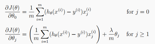
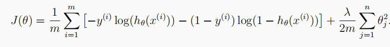
1.3.1 Cost function

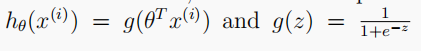
The cost function of regularized logistic regression is:

1.3.2 Gradient

The gradient descent method of regularized logistic regression cost function is expressed as follows, because there is no penalty t h e t a 0 theta_0 theta0, so it can be divided into two cases:

1.4 One-vs-all Classification

In this part, we will train multiple regularized logistic regression classifiers to realize "one to many classification", and each category corresponds to the data set K K One of class K.

For this task, we have 10 possible classes, and because logistic regression can only classify between two classes at one time, each classifier is determined between "belonging to category i" and "not belonging to category i". We will include classifier training in a function that calculates the final weight of each of the 10 classifiers and returns the weight to shape ( k , ( n + 1 ) ) (k, (n+1)) (k,(n+1)), where n n n is the number of parameters.

# 1.4 one vs all classification
all_theta = func.oneVsAll(X, y, l=1, K=10)
predictions = func.predictOneVsAll(X, all_theta)
accuracy = np.mean(predictions == y)
print('accuracy = ' + format(accuracy * 100) + '%')

there h h h total 5000 5000 5000 lines, 10 10 10 columns, each row represents a sample, and each column is the probability of predicting the corresponding number. We take the subscript corresponding to the maximum probability plus 1 1 1 is the category finally predicted by our classifier. In addition, the final return h _ a r g m a x h\_argmax h_argmax is an array containing 5000 5000 The predicted value corresponding to 5000 samples.

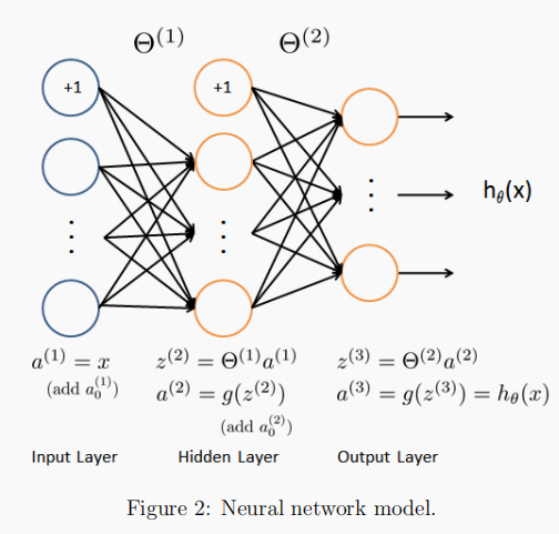
2. Neural Networks

This section includes some details of exploring "neural networks".

• The relevant functions called are described in detail in the article header "self created functions".

The first chapter uses multi class logistic regression. However, logistic regression cannot form more complex assumptions because it is only a linear classifier.

Next, we use neural network to try. Neural network can realize very complex nonlinear model. We will use the trained weights for prediction.

# 2. Neural Networks
path = '../data/ex3weights.mat'
theta1, theta2 = func.loadWeight(path)
print(theta1.shape)
print(theta2.shape)

2.1 Model Representation

The training sample X gradually increases from 1 to train different parameter vectors θ. Then, the validation error is calculated by cross validation sample Xval.

1. Use the subset of training set to train the model and get different results θ.
2. adopt θ When calculating the training cost and cross validation cost, remember not to use regularization at this time λ = 0 λ=0 λ=0.
3. When calculating the cross validation cost, remember to calculate the whole cross validation set without dividing it into subsets.

# 2.1 Model Representation
X, y = func.loadData('ex3data1.mat')
X = np.insert(X, 0, values=np.ones(X.shape[0]), axis=1)
y = y.flatten()

2.2 Feed Forward Propagation and Prediction

# 2.2 Feedforward propagation and prediction
# Every hidden layer should be inserted with a bias unit

# Input layer
a1 = X

# Hidden layer
z2 = a1 @ theta1.T
z2 = np.insert(z2, 0, 1, axis=1)
a2 = func.sigmoid(z2)

# Output layer
z3 = a2 @ theta2.T
a3 = func.sigmoid(z3)

# Make predictions
y_predictions = np.argmax(a3, axis=1) + 1
accuracy = np.mean(y_predictions == y)
print('accuracy = ' + format(accuracy * 100) + '%')