1, Overview
The single factor model was first proposed by William sharp. The basic idea of the single factor model is that the securities return is affected by only one factor. Market model is a typical example of this model.
If we observe the stock market, we will find that when the market stock index rises, most stock prices rise at the same time; vice versa. This shows that all kinds of securities have a linkage response to a factor, that is, the change of market stock price index.
Two, model formula
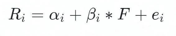
Where F is the predicted value of the common factor, and beta is the sensitivity of securities i to the factor.
3, Implement a small strategy
Take the stocks of SSE 50 as the stock pool, manually select a factor, sort the stocks according to the value of the factor, buy the stocks in front, and adjust the position every week.
# coding=utf-8
from __future__ import print_function, absolute_import
from gm.api import *
from gm.enum import OrderSide_Sell, OrderType_Market
import numpy as np
import pandas as pd
'''
Stock pool: 50 stocks in SSE 50
 Select stock pool BP The top five stocks with factor values,
Position adjustment is carried out every month. If the top five stocks do not have positions, they will buy, and if they have positions, they will continue to hold positions
'''
# There must be an init method in the policy
def init(context):
    context.index = 'SHSE.000016'
    context.num = 5  # The top five stocks are entrusted for position adjustment
    schedule(schedule_func=algo_1, date_rule='1w', time_rule='09:31:00')

def algo_1(context):
    now = context.now
    # Acquire 50 constituent shares of SSE
    symbols = get_history_constituents(index='SHSE.000016',
                                       start_date=now,
                                       end_date=now)[0].get('constituents').keys()
    # Obtain the constituent stocks composed of SSE 50 on the current date and extract its factor data
    DF = get_fundamentals_n(table='trading_derivative_indicator',
                            symbols=symbols,
                            end_date=now,
                            count=1,
                            fields='PB',
                            df=True)
    # Calculate the book to market ratio, which is the reciprocal of P/B
    DF['PB'] = (DF['PB'] ** -1)
    # Rank stocks according to factor data
    df = DF.sort_values(['PB'], ascending=False)
    target_list = df['symbol'].values[:context.num]

    # Designated position
    # Get all existing positions
    pos_all = context.account().positions()
    #For the subject matter of position, if it is not in the screened stock pool, the subject matter shall be eliminated
    for i in pos_all:
        if i['symbol'] not in target_list:
            order_volume(symbol=i['symbol'], volume=i['available'], side=OrderSide_Sell, order_type=OrderType_Market, position_effect=PositionEffect_Open)
            print("To liquidate shares not included in the underlying stock:",i['symbol'],"Quantity is",i['available'])


    for symbol in target_list:
        pos = context.account().position(symbol=symbol,side = PositionSide_Long)
        #If the target is not in the position, open the position
        if not pos:
            order_target_percent(symbol=symbol, percent=1/context.num,
                                position_side=PositionSide_Long, order_type=OrderType_Market)
            print("Stock purchased at market price:",symbol)


if __name__ == '__main__':
    run(strategy_id='xxxxxxxxxxx',
        filename='main.py',
        mode=MODE_BACKTEST,
        token='xxxxxxxxxxxxxx',
        backtest_start_time='2020-11-01 08:00:00',
        backtest_end_time='2021-11-20 16:00:00',
        backtest_adjust=ADJUST_PREV,
        backtest_initial_cash=10000000,
        backtest_commission_ratio=0.0001,
        backtest_slippage_ratio=0.0001)
4, Single factor test
Here we often use the following three methods: grouping back test, information coefficient evaluation and regression test. The following contents will explain the contents of these three methods, in which the codes of information coefficient evaluation and regression test will be given. Please improve the grouped back test~
1. Group backtesting:
Back test method quantile
Sort the stocks according to the factor size, divide the stock pool into N combinations, or divide them equally in each industry.
Each equity is generally equal to the right of choice. The inter industry weight is generally the same as the industry ratio of the benchmark (such as CSI 300). At this time, the combination is industry neutral.
By grouping the cumulative return graph, we can simply know whether the factor is monotonically increasing or decreasing with the rate of return.
2. Information coefficient evaluation:
Information Coefficient (IC for short) refers to the cross-sectional correlation coefficient between the factor value of the selected stock and the stock return in the next period. Through the IC value, the prediction ability of the factor value to the return in the next period can be judged.
The IC value can well reflect the prediction ability of the factor. The higher the IC, the stronger the prediction ability of the factor to the stock return in this period. Generally, if the IC is greater than 3% or less than - 3%, the factor is considered to be more effective.
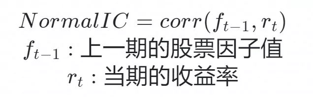
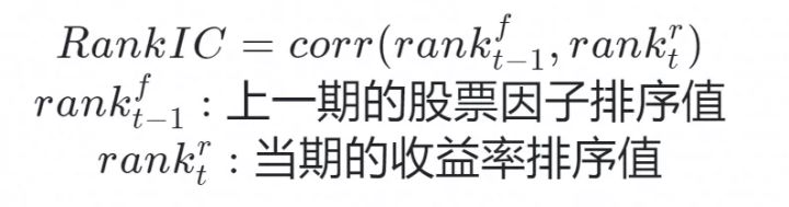
There are two common ICs, one is Normal IC (the concept of quasi Pearson correlation coefficient) and the other is Rank IC (quasi pearman correlation coefficient).
- Normal IC: the cross-sectional correlation coefficient between the exposure value of a factor in all stocks at a certain point in time and its return in the next period.
- Rank IC: the cross-sectional correlation coefficient between the ranking of a factor in all stock exposure values at a certain point in time and its ranking of returns in the next period.
For example, we need to calculate the factor Normal IC value of the current time, and its code is as follows:
import datetime
#Get current date and time
now_time = datetime.datetime.now()
#format
now_time=now_time.strftime('%Y-%m-%d')
# Acquire 50 constituent shares of SSE
symbols = get_history_constituents(index='SHSE.000016',
start_date=now_time,
end_date=now_time)[0].get('constituents').keys()
# Obtain the constituent stocks composed of SSE 50 on the current date and extract its factor data
DF = get_fundamentals_n(table='trading_derivative_indicator',
symbols=symbols,
end_date=now_time,
count=1,
fields='PB',
df=True)
# Calculate the book to market ratio, which is the reciprocal of P/B
#2021.8. Factor exposure value of 25
yz=DF['PB']
#2021.8. 25 stock return, 8.25 stock return -8.24 closing price / 8.24 closing price
a=[]
for i in DF['symbol']:
history_n_data = history_n(symbol=str(""+i+""), frequency='1d', count=2, end_time='2021-10-25', fields='close', adjust=ADJUST_PREV, df=True)
a.append((history_n_data['close'][1]-history_n_data['close'][0])/history_n_data['close'][0])
np.corrcoef(a,yz)
#The results are as follows:
#array([[1. , 0.17563877],
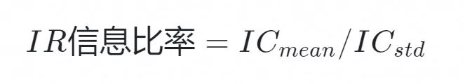
# [0.17563877, 1. ]])IR information ratio:
IR information ratio is the mean of IC divided by standard deviation, that is, the information ratio of IC value in the back test time period. The Alpha excess return acquisition ability of the factor can be evaluated, and it is a more stable acquisition ability.
In view of the importance of IC, the IC mean weight of the factor in the last N months (default 12) is often used in multi factor factor weighting, and the result is usually better than the equal weight method.
IC_IR evaluation:
1) Rank IC value series mean one factor significance;
2) One factor stability of standard deviation of Rank IC value series;
3)IC_IR (ratio of mean to standard deviation of Rank IC value series) one factor validity;
4) Whether the proportion of Rank IC value sequence greater than zero is stable.
The codes of the main methods are as follows:
# Calculate the IC absolute value mean, positive proportion, mean / standard deviation of a group of data
def ics_return(l):
# Mean value of absolute value of information coefficient
a = [abs(i) for i in l]
avr_ic = sum(a) / len(l)
# Information proportion
b = np.array(l)
if b.std() != 0:
ir = b.mean() / b.std()
else:
ir = 0
# Positive proportion
c = [i for i in l if i > 0]
pr = len(c) / len(l)
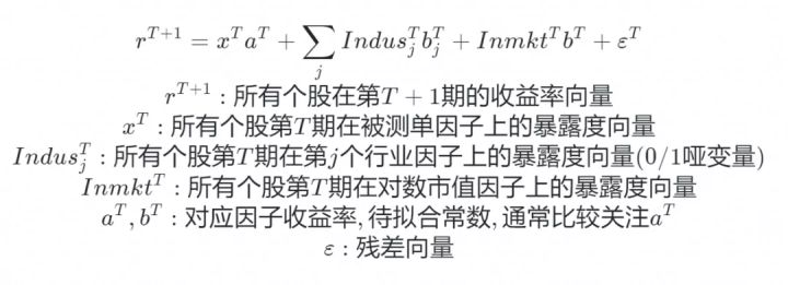
return avr_ic, ir, pr3. Regression test:
The specific method is to conduct linear regression between the factor exposure vector in phase t and the stock return vector in phase T+1. The obtained regression coefficient is the factor return of the factor in phase t, and the significance level t value of the factor return in the regression of this period can also be obtained.
Generally, when the absolute value of t value is greater than 2, the factor is more effective.
The factor exposure of individual stocks in a certain cross-sectional period refers to the factor value of individual stocks on this factor at the current time.
Calculation method:
Regression factor evaluation:
1) t-value sequence is an important criterion for the significance of absolute value mean factor;
2) The proportion of absolute value of t-value sequence greater than 2 - judge whether the significance of the factor is stable;
3) The combination of t-value sequence mean value 1 and a. can judge whether the positive and negative direction of factor t is stable;
4) Mean value of factor return series - judge the size of factor return.
# t-test value of coefficient of linear regression equation
def t_value(x, y):
    x2 = sum((x - np.mean(x)) ** 2)
    xy = sum((x - np.mean(y)) * (y - np.mean(y)))

    #Least squares estimation of regression parameters
    beta1 = xy / x2
    beta0 = np.mean(y) - beta1 * np.mean(x)
    #Output linear regression equation
    # print('y=',beta0,'+',beta1,'*x')

    #variance
    sigma2 = sum((y - beta0 - beta1 * x) ** 2) / len(x)
    #standard deviation
    sigma = np.sqrt(sigma2)
    #Find the value of t
    t = beta1 * np.sqrt(x2) / sigma
    return t
The above is all today's content. If there are deficiencies, please forgive me ~ welcome to leave a message below and pass it Nuggets community Share personal quantitative experience! In the future, we will launch other series of articles one after another. Please look forward to it~
Statement: this content is first to nugget quantification official account, which is used for learning, communication and demonstration, and does not constitute any investment suggestion. If you need to reprint the original article, please contact Nuggets Q (myquant2018)