catalog
3.2 Otsu method with multiple thresholds
3.3 multi threshold Otsu method 2
4.2.1 single location and single point crossing
4.2.2 multi position and single point crossing
8.1 test script ga_muti_thresholding.m
8.2 population initialization init_pop.m
8.6 calculation of fitness function_ fit.m
1. Summary
Image segmentation is an important problem in image processing and computer vision, and it is the key step of image processing and analysis. Image segmentation is to divide a digital image into multiple regions or sets. In order to solve the problem of time-consuming in traditional image thresholding segmentation method and make full use of the high efficiency of genetic algorithm, a multi thresholding image segmentation method based on genetic algorithm is proposed, which takes the maximum between class variance or the minimum within class variance as an important reference standard. Experimental results show that the genetic algorithm can not only achieve image threshold segmentation, but also reduce the segmentation time significantly.
Keywords: image segmentation genetic algorithm multi threshold segmentation
2. Introduction
In a broad sense, image segmentation is to divide image into sub regions or objects according to image components, and the way of image segmentation depends on the problem we want to solve; the ultimate goal of segmentation is to extract the part we are concerned about from the image, so as to further research, analysis and processing, and the accuracy of image segmentation stage will be for the image in the next stage The management effect has a great influence. For many applications that rely on computer vision, such as medical imaging, target location in satellite images, machine vision, fingerprint and face recognition, agricultural imaging, etc., it is an essential preprocessing task.
Therefore, image segmentation has been studied for many years. At present, the commonly used image segmentation methods are: Based on threshold segmentation, edge segmentation, region segmentation, based on wavelet, genetic algorithm, artificial neural network, active contour model, clustering segmentation and so on [1]. Among them, because of the simplicity of threshold segmentation technology, and threshold method is the most common parallel direct detection area segmentation method. The key step is how to select threshold, which has been widely concerned in recent years. Many threshold selection methods have been proposed. For example, Otsu algorithm, minimum error threshold method and best histogram entropy method. On the other hand, because genetic algorithm can provide near optimal solutions for many practical applications, the problem of finding the optimal threshold is transformed into an optimization problem in a finite field.
In this paper, the threshold segmentation method is combined with genetic algorithm. Based on the threshold segmentation method to maximize the variance between different regions or objects, this method is called Otsu algorithm. This standard is used as the fitness standard of genetic algorithm to search the best threshold.
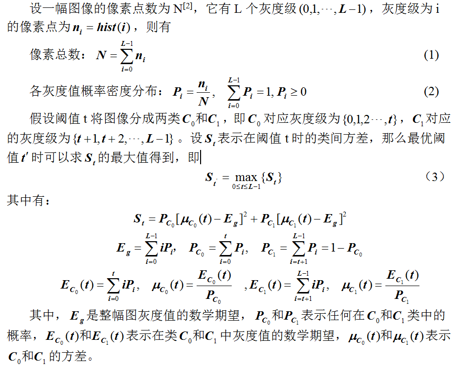
3 Otsu threshold segmentation
Otsu algorithm, also known as Otsu method, is an algorithm to determine the threshold value of image binary segmentation, which was proposed by Japanese scholar Otsu in 1979. In terms of the principle of Dajin method, it is also called the method of maximum inter class variance. This method is considered to be the best algorithm for threshold selection in image segmentation. It is simple to calculate and not affected by image brightness and contrast, so it has been widely used in digital image processing. Its basic principle is to use the best threshold to divide the gray histogram into two parts, so that the variance between the two parts is the maximum, that is, the maximum separation. The classical Otsu method can only be used for single threshold segmentation. In the process of thresholding segmentation, the information hist(x) of gray histogram is mainly used to calculate.
3.1 classical Otsu method
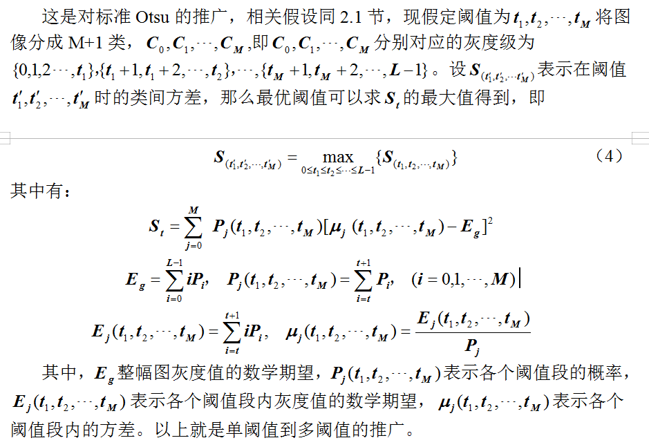
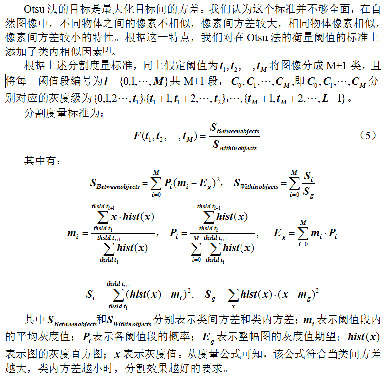
3.2 Otsu method with multiple thresholds
3.3 multi threshold Otsu method 2
4 genetic algorithm design
Genetic algorithm (GA) is a heuristic search algorithm which simulates the genetic and evolutionary process of organisms in the natural environment to form an adaptive global optimization probability [4]. Genetic algorithm is a population-based algorithm, which generates multiple solutions each iteration. When there is no deterministic method or the computational complexity of deterministic method, genetic algorithm is used to search the optimal solution. It has two significant advantages: implicit parallelism and effective use of global information, which is helpful to improve the search speed and robustness of the algorithm. Combined with image segmentation based on multi threshold, the genetic algorithm is designed as follows:
4.1 individual code
In genetic algorithm, the population evolves through continuous iterations. We may think that an individual has only one chromosome, that is, the individual is equal to the chromosome, in which each chromosome corresponds to a solution of the problem, and the individual evolution is equal to the final result of chromosome crossing, mutation and survival of the fittest. Because the common threshold segmentation will preprocess the image. Color image, each pixel has three values (RGB), each value range is 0 ~ 255. Gray image, each pixel has only one value, called gray value. Because processing gray image is simpler and more efficient than processing color image. Therefore, the preprocessing is to convert the color image to the gray image, and each pixel value is in [0255]. Because each threshold is a gray value, each threshold is defined as a binary bit vector with a length of L, and each binary bit is called a gene, where l = log (gray value series); for n threshold, each chromosome contains n*L binary bits, where each L bit represents a threshold, and the chromosome structure is shown in Figure 1 below.
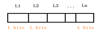
Figure 1: chromosome structure
4.2 mating operation
Mating can also be understood as the crossing between chromosomes. The chromosomes perform the crossing operation at random points. The following introduction will use the single point crossing method:
4.2.1 single location and single point crossing
Take the whole chromosome as a unit, randomly generate a random number in the range of 1~L*n, take this point as the beginning of chromosome crossing operation, and successively exchange the following bits (genes). The specific operation is shown in Figure 2.
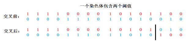
Figure 2: single point chromosome crossing at crossing position 14
4.2.2 multi position and single point crossing
The L-bit binary encoding of each threshold within the chromosome is taken as the unit. If a chromosome contains n thresholds, then n cross random values are randomly generated, and the random values range from 1 to log (gray scale Series). The thresholds of the corresponding positions of the two chromosomes were crossed at one point. The specific operation is shown in Figure 3.
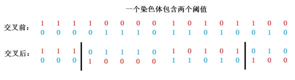
Figure 3: Multipoint chromosome crossing at 4 and 14, respectively
4.3 variation operation
Variation is the change (reversal) of a gene's position, which is used to overcome the possible local optimum caused by crossing. The specific method of a mutation is to randomly generate a random number, the random number range is 1~n*L, and flip the binary bit on the position.
4.4 selection operation
The selection operation is very important in genetic algorithm. According to the fitness of each individual, the most suitable individual is selected to keep to the next generation. At the same time, the individual with low fitness is also selected. Therefore, the roulette method is used for selection. Through the fitness value of each individual, the probability = individual fitness value / population overall fitness sum is calculated, and then the cumulative probability is calculated according to the above. The probability of each individual being selected = individual cumulative probability / total group cumulative probability. This is a normalization process, and each individual is allocated to the roulette with probability of 1 in proportion. In order to improve the convergence speed and increase elite retention, the superior individuals of the parents will replace the inferior individuals of the newly selected offspring.
Select n individuals to form the next generation population, and the specific operation is as follows:
(a) Calculate the individuals with the best adaptability of their parents.
(b) Calculate the cumulative probability of each individual in the parent generation.
(c) Generate n random numbers between 0 and 1.
(c) According to the cumulative probability, the first individual larger than the random number is selected.
(e) The superior individuals of the parents will replace the inferior individuals of the new offspring.
3.5 fitness function setting
For the fitness evaluation of threshold segmentation, that is, what kind of threshold segmentation can separate the object and what kind of segmentation is good. In this paper, Otsu's maximum inter class variance or minimum intra class variance is used as the threshold segmentation criteria. For different thresholds, the larger the variance between classes and the smaller the intra class variance, the better the segmentation effect.
5 Analysis of test results
The test is implemented in Matlab environment. The parameter settings are as follows:
Population size: 20
Cross probability: 0.8
Probability of variation: 0.1
Maximum iterations: 100
5.1 test one
(a) (b)
(c ) (d)
Figure 4: (a) original cell picture [5]; (b) effect picture after threshold segmentation; (c) gray histogram of original picture; (d) segmentation red line with threshold value of 210 divides gray value histogram into two parts
5.2 test II
(a) (b)
(c) (d)
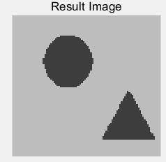
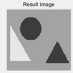
Figure 5: (a) the original building block picture; (b) the grayed image; (c) an effect picture with a segmentation threshold of 123 gray value segmentation; (d) an effect picture with two segmentation thresholds of 119 and 207 gray value segmentation, respectively
Because the threshold used for segmentation is less than the object type, some object objects will be defined as the background, only the object with the largest gray difference will be used as the distinguishing object, which is suitable for highlighting some of the most important objects in the multi object image. When the number of segmentation thresholds is equal to or greater than the object type, all different object objects in the image can be distinguished as well as possible.
Table 1: comparison between traditional Otsu method and genetic algorithm (see Figure 5 for effect object)
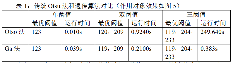
It can be seen from table 1 that in the case of single threshold, traditional Otsu traverses all pixels (256), and calculates the class variance corresponding to each pixel value respectively, which is very fast, faster than genetic algorithm. However, when multi threshold segmentation is implemented, the number of iterations will increase exponentially due to the number of thresholds, which makes the running time of the program too long and reduces the efficiency.
5.3 test three
(a) (b)
(c)
(d)
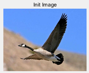
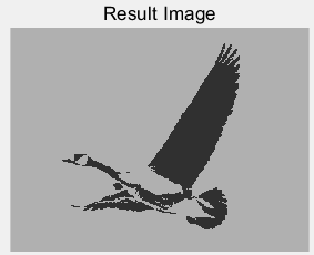
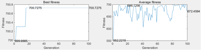
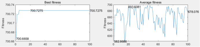
Figure 6: (a) the original bird map; (b) the bird map segmented by the threshold value of 97 gray level; (c) the best adaptability and average adaptability of each generation of single point crossing; (d) the best adaptability and average adaptability of each generation of multi point crossing
Table 2: comparison of two different cross methods mentioned in the paper (the effect of the object is shown in Figure 6)
|
Cross mode |
Optimal threshold |
Achieve the best Threshold algebra |
Reach the best threshold Time taken by value |
Complete operation Line time |
|
Single point crossing |
97 |
12 |
0.122s |
0.2190s |
|
Multipoint crossing |
97 |
22 |
0.125s |
0.2860s |
From table 2, it can be seen that single point intersection can converge earlier and take less time overall. As each threshold in the multi-point cross operation increases the cross operation and time consumption, it can be seen from the average fitness of each generation in the right figures (c) and (d) of Figure 6 that the multi-point cross jitter is more obvious. It is to spend more time to expand the search space to reduce the possibility of falling into local optimum.
5.4 test four
(a) (b)
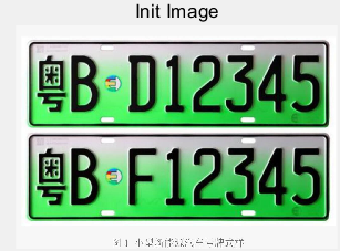
Figure 7: (a) the original license plate image; (b) the license plate image segmented by the threshold value of 123
Table 3: comparison of two calculation methods of fitness mentioned in the paper (see Figure 7 for effect object)
|
Fitness criteria |
Optimal threshold |
Reach optimal threshold algebra |
Reach the best threshold Time taken by value |
Complete operation Line time |
|
Maximize between classes |
123 |
11 |
0.0320s |
0.2600s |
|
Maximizing between classes & minimizing within classes |
124 |
10 |
0.0270s |
0.2220s |
From table 3, it can be seen that the effect of the two segmentation methods is similar, and the fitness strategy of maximizing combination within classes and minimizing between classes runs faster.
6 Conclusion
Thresholding based segmentation is a deterministic but very complex problem. Compared with the traditional Otsu method, genetic algorithm is used to search for the optimal solution through the heuristic information between populations, so as to quickly approach the optimal solution, which can greatly improve the efficiency of finding the optimal solution, and the efficiency is considerable. At the same time, for different scenes, using different threshold number, we can effectively extract the important object individuals in the image.
7. Reference
[1] Ding Liang, Zhang Yongping, Zhang Xueying. Overview of image segmentation methods and pre performance evaluation [J]. Software. 2010 (12): 78-83
[2] Liu Jianzhuang, Xie Weixin, Gao Xinbo. Genetic algorithm for multi threshold image segmentation [J]. Pattern recognition and artificial intelligence. 1995.12:126-132
[3]Omar B, Yahya A Y.Multi-Thresholding Image Segmentation Using Genertic Algorithm[J].Computer Vision.,59(2),2004:167-181.
[4] Ma Wen, Zhou Shaoguang, Ding Huizhen. Application of Otsu method based on Genetic Algorithm in image segmentation [J]. Coastal enterprises and technology. 2005 (8): 160-162
[5]CSDN blog. Application of Ostu method based on Genetic Algorithm in image segmentation [OL] https://blog.csdn.net/u010945683/article/details/41780491
8 code part
8.1 test script ga_muti_thresholding.m
%
% Muti-Thresholding Image Segemention Using Genetic Algonithm
% Multi threshold image segmentation based on genetic algorithm
% Author:
% data : 2020/06/03
% Objective: to maximize the inter class variance between the target and the background or to minimize the inter class variance within the target pixel
% Encoding: binary encoding determines the number of bits according to the range of gray value thsld_len According to the number of preset thresholds thsld_mount
% The length of each chromosome is determined as: thsld_len*thsld_mount
% Fitness function:
% Choice: Roulette
% Variation: single point variation
%%
%(0) empty
clc;
clear;
close all;
%%
%(1) Determine parameters
pop_size = 20; %Population size
pc = 0.8; %Crossover probability
pm = 0.1; %Mutation probability
iter_max = 100; %Maximum number of iterations
thsld_mount = 3; %Number of thresholds
thsld_len = log2(256); %Bits per threshold
image_path = '14.jpg'; %Image path
compression_ratio = 0.4; %Image compression ratio
elite_pro = 0.1; %Proportion of parents in elite retention
%%
%(2)Image preprocessing
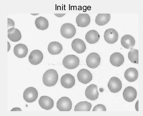
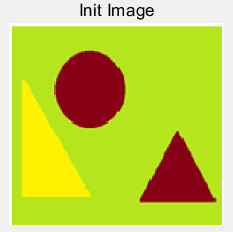
init_image = imread(image_path); %Read in picture
subplot(3,3,1);
imshow(init_image);
title('Init Image');
%Reduce the number of pixels, reduce the amount of calculation and improve the efficiency of calculation
compress_image = imresize(init_image,compression_ratio); %Reduce the picture to 0% of the original picture.2 times
subplot(3,3,2);
imshow(compress_image);
title('Compress Image');
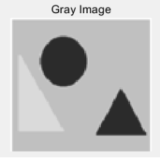
%The quality of segmentation is affected by the uniformity of gray value of each target pixel, and graying is helpful to reduce the influence
gray_image = rgb2gray(compress_image); %Color image graying
subplot(3,3,3);
imshow(gray_image);
title('Gray Image');
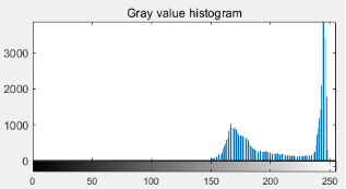
hist = imhist(gray_image); %Generating histogram data from gray image
subplot(3,3,4);
imhist(gray_image);
title('Gray value histogram');
%%
t_start = clock;
%Code logic part
%Initial population
pop = init_pop(pop_size,thsld_mount);
%Keep records
history = zeros(iter_max,2); %Best fitness value of each generation average fitness value of each generation
history_pop = zeros(iter_max,thsld_mount); %The best fit threshold of each generation the average value of each threshold segment of each generation
%Maximum iteration within algebra
flag = ceil(iter_max * (1-0.4));
tim = zeros(iter_max,6)
for iter = 1:iter_max
%overlapping
cross_pop = crossing(pop,pc,thsld_len);
%variation
muta_pop = mutation(cross_pop,pm,thsld_len);
%choice
[pop best_fit_aver_fit cur_best_pop ] = selection(pop,muta_pop,thsld_mount,hist,elite_pro);
history(iter,:) = best_fit_aver_fit;
history_pop(iter,:)= cur_best_pop;
tim(iter,:) = clock;
fprintf("%d:best fitness:%f\n",iter,history(iter,1));
fprintf("%d:best pop answer:%s\n\n",iter,num2str(history_pop(iter,:)));
%Adjust selection and compilation probability
if iter == flag
pc = pc * 0.4;
pm = pm * 0.4;
end
end
t_end = clock;
%% Graph output results
subplot(3,3,5);
plot(history(:,1));
title('Best fitness');
xlabel('Generation');
ylabel('Fitness');
text(1,history(1,1),num2str(history(1,1)));
text(20,history(20,1),num2str(history(20,1)));
text(iter_max,history(iter_max,1),num2str(history(iter_max,1)));
subplot(3,3,6);
plot(history(:,2));
title('Average fitness');
xlabel('Generation');
ylabel('Fitness');
text(1,history(1,2),num2str(history(1,2)));
text(20,history(20,2),num2str(history(20,2)));
text(iter_max,history(iter_max,2),num2str(history(iter_max,2)));
subplot(3,3,7);
plot(history_pop);
title('Thlsd value');
xlabel('Generation');
ylabel('Thlsd value');
for t = 1:thsld_mount
text(iter_max-10,history_pop(iter_max-10,t),num2str(history_pop(iter_max-10,t)));
end
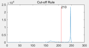
subplot(3,3,8);
plot(hist);
title('Cut-off Rule');
hold on
y = max(hist);
color = ['r','g','b','c','y','m','b'];
for t = 1:thsld_mount
pos = rem(t,7);
if pos == 0
pos = 7;
end
plot([history_pop(iter_max,t),history_pop(iter_max,t)],[0,y],color(pos));
text(history_pop(iter_max,t),y-(t*100),num2str(history_pop(iter_max,t)));
end
%Redraw
last_thsld = history_pop(iter_max,:);
[row list ]= size(gray_image);
%Determine the color value of each interval segment
color = zeros(1,thsld_mount+1);
for i=1:thsld_mount+1
if i == 1
color(1) = uint8(fix((1 + last_thsld(1)-1)/2));
elseif i < thsld_mount+1
color(i) = uint8(fix((last_thsld(i-1) + last_thsld(i)-1)/2));
else
color(i) = uint8(fix((last_thsld(i-1) + 256)/2));
end
end
new_image = zeros(size(gray_image));
for i = 1:row
for j = 1:list
for k = 1:thsld_mount+1
if k == thsld_mount+1
new_image(i,j) = color(k);
elseif gray_image(i,j) < last_thsld(k)
new_image(i,j) = color(k);
break;
end
end
end
end
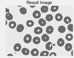
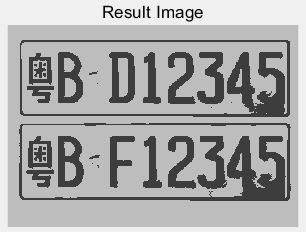
subplot(3,3,9);
imshow(uint8(new_image));
title('Result Image');
run_time = etime(t_end,t_start);
disp(run_time);8.2 population initialization init_pop.m
function pop = init_pop(pop_size,thsld_mount)
%Random generation[0 255]Decimal threshold between
pop = zeros(pop_size,thsld_mount);
for i = 1:pop_size
    pop(i,:) = randperm(256,thsld_mount);
end
end
8.3 cross operation
function cross_pop = crossing(pop,pc,thsld_len)
[row list] = size(pop);

%Single point intersection of multiple intersections

%Calculate how many individuals need to cross
cross_mount = fix( row * pc ) ;        %Round down
if rem( cross_mount,2) ~= 0            %Make even numbers convenient for crossing
    cross_mount = cross_mount + 1;     %Since it starts to round down, plus 1 doesn't worry about crossing the border
end
%Random sampling from population cross_mount Individuals mating
cross_num = randperm(row,cross_mount);       %From 1~row Medium, select cross_mount Do not repeat random arrangement
% fprintf('cross_num:%s\n',num2str(cross_num));
%Make a twofold crossing
for i = 1:2:cross_mount
    %Single point crossing for each threshold
    while 1
        %Each threshold component has different degree of single point crossing
        cross_pos = randi(thsld_len,1,list);
        %Encode decimal to binary
        x = dec2base(pop(cross_num(i),:),2,thsld_len);   %8 String array represented by bit 2
        y = dec2base(pop(cross_num(i+1),:),2,thsld_len);
        for j = 1:list
            for k=cross_pos(j):thsld_len
                temp = x(j,k);
                x(j,k) = y(j,k);
                y(j,k) = temp;
            end
        end
        %Convert binary to decimal
        pop(cross_num(i),:) = base2dec(x,2)';
        pop(cross_num(i+1),:) = base2dec(y,2)';
        %Check whether the same threshold value is generated in a descendant
        ux = length(pop(cross_num(i),:))-length(unique(pop(cross_num(i),:)));
        uy = length(pop(cross_num(i+1),:))-length(unique(pop(cross_num(i+1),:)));
        if ux == 0 && uy == 0 && sum(pop(cross_num(i),:)>256)==0 ...
                  && sum(pop(cross_num(i+1),:)>256)==0
            break;
        end
    end
%Single point crossing with only one intersection
%       while 1
%           r = randi(list * thsld_len,1);
%           %Encode decimal to binary
%           x = dec2base(pop(cross_num(i),:),2,thsld_len);   %8 String array represented by bit 2
%           y = dec2base(pop(cross_num(i+1),:),2,thsld_len);
%
%           cross_row = ceil(r/(thsld_len));
%           if rem(r,thsld_len) == 0
%               cross_list = thsld_len;
%           else
%               cross_list = rem(r,thsld_len);
%           end
%
%           for j = cross_row:list
%               if j == cross_row   %Cross the data of the current row first
%                   for k = cross_list:thsld_len
%                       temp = x(j,k);
%                       x(j,k) = y(j,k);
%                       y(j,k) = temp ;
%                   end
%               else
%                 for k = 1:thsld_len   %Cross other row data
%                       temp = x(j,k);
%                       x(j,k) = y(j,k);
%                       y(j,k) = temp;
%                 end
%               end
%           end
%
%           %Convert binary to decimal
%           %Check whether the same threshold value is generated in a descendant
%           ux = length(pop(cross_num(i),:))-length(unique(pop(cross_num(i),:)));
%           uy = length(pop(cross_num(i+1),:))-length(unique(pop(cross_num(i+1),:)));
%           if ux == 0 && uy == 0 && sum(pop(cross_num(i),:)>256)==0 ...
%                   && sum(pop(cross_num(i+1),:)>256)==0
%               break;
%           end
%       end
% end
cross_pop = pop;
end
8.4 mutation.m
function muta_pop = mutation(pop,pm,thsld_len)
[row list] = size(pop);
muta_mount = ceil(row * list * thsld_len * pm);   %Calculate the total number of binary digits to be varied
muta_num = randperm(row * list * thsld_len,muta_mount);

for i = 1:muta_mount
    % muta_num(i)
    muta_row = ceil(muta_num(i) / (list * thsld_len));
    if rem(muta_num(i),list * thsld_len) == 0
        muta_list = list;
    else
        muta_list = ceil(rem(muta_num(i),list * thsld_len) / thsld_len);
    end
    %
    %Encode decimal to binary
    z = dec2base(pop(muta_row,muta_list),2,thsld_len);   %8 String array represented by bit 2
    if rem(muta_num(i),list * thsld_len) == 0
        muta_bit = thsld_len;
    else
        muta_bit = rem(muta_num(i),list * thsld_len) - (muta_list-1) * thsld_len;
    end
    while 1
        if z(muta_bit) == '0'
            z(muta_bit) = '1';
        else
            z(muta_bit) = '0';
        end
        pop(muta_row,muta_list) = base2dec(z,2);
        %Check whether there is the same threshold in an individual after mutation
        uz = length(pop(muta_row,:))-length(unique(pop(muta_row,:)));
        if uz == 0 && sum(pop(muta_row,:)>256)==0
            break;
        else
            muta_bit = randi(thsld_len,1);
        end
    end
end
muta_pop = pop;
end
8.5 selection.m
function [select_pop best_fit_aver_fit cur_best_pop] = selection(pop,new_pop,thsld_mount,hist,elite_pro)

[row list] = size(pop);
%Check threshold changed to 0 by mutation or crossover
new_pop(new_pop==0)=1;

f_num = ceil(elite_pro * row) ;

temp_pop = zeros(size(pop));
select_fit = zeros(1,row);
%30%Keep the excellent individuals of the parents
f_fitness = compute_fit(pop,hist);
[a b] = sort(f_fitness,'descend');
temp_pop = pop(b(1:f_num),:);
select_fit = f_fitness(b(1:f_num));

%Calculate offspring fitness
s_fitness = compute_fit(new_pop,hist);

%Calculate the cumulative probability according to the fitness value
cumulat_fit = zeros(row,1);    %Cumulative fitness
pro = zeros(row,1);            %Cumulative probability
c_sum = 0;

for i = 1:row
    c_sum = c_sum + s_fitness(i);
    cumulat_fit(i) = c_sum;
end
por = cumulat_fit/c_sum;

%roulette wheel selection  row - f_num Individuals
s_num = row - f_num;
[a b] = sort(s_fitness,'descend');
temp_pop(f_num+1:row,:) = new_pop(b(1:s_num),:);
history_j = zeros(1,row);
for i=1:s_num
    r = rand;
    for j=1:row
        if por(j) >= r
            history_j(i) = j;
            temp_pop(f_num+i,:) = new_pop(j,:);
            select_fit(f_num+i)= s_fitness(j);
            break;
        end
    end
end

%Best and average fitness of each generation after selection
best_fit = max(select_fit);
aver_fit = mean(select_fit);
best_fit_aver_fit = [best_fit aver_fit];

%The solution space of the best fitness after selection
[a b] = sort(select_fit,'descend');
cur_best_pop = temp_pop(b(1),:);
select_pop =temp_pop;
end
8.6 calculation of fitness function_ fit.m
%% (4)Calculation of fitness

%Fitness 2
% function fitness = compute_fit(pop,hist)
% [row list] = size(pop);
%
% %Sort each individual and then adjust it back
% [sort_pop order] = sort(pop,2);
%
% %(4.1)Calculate variance between classes
% %(4.1.1)Calculate the average value of pixels in the threshold segment
% m = zeros([row list+1]);
% %(4.1.2)Calculate the probability within the threshold segment
% p = zeros([row list+1]);
% %(4.1.3)Calculate global pixel average
% mg = zeros(row,1);
% sum_i = zeros([row list+1]);
% for k = 1:row     %row Individuals
%     for i=1:list+1
%         %Determine threshold segment start
%         if i == 1
%             m_start = 1;
%         else
%             m_start = pop(k,i-1);
%         end
%         %Determine threshold segment start
%         if i == list+1
%             m_end = 256;
%         else
%             m_end = pop(k,i)-1;
%         end
%
%         for j = m_start:m_end
%             m(k,i) = m(k,i) + j * hist(j);           %Common understanding: total gray level in threshold segment
%             sum_i(k,i) = sum_i(k,i) + hist(j);       %General understanding: the total number of pixels in the threshold segment
%         end
%     end
%     sum_i(k,sum_i(k,:)==0) = 0.0001;
%     m(k,:) = m(k,:)./sum_i(k,:);              %Average gray level of pixels in threshold segment
%     p(k,:) = sum_i(k,:)./sum(sum_i(k,:));     %Probability of pixel number of each threshold segment in total pixel number
% end
% mg = sum(m.*p,2);                %Expectation of overall gray value of each individual  row * 1
% S_bo = sum(p .* ((m - mg) .^ 2),2);    %Between objects variance  row*1
%
% %(4.2)Calculate intra class variance
% %(4.2.1)Calculate variance within threshold segment Si
% si = zeros([row list+1]);
% for k = 1:row     %row Individuals
%     for i=1:list+1
%         %Determine threshold segment start
%         if i == 1
%             m_start = 1;
%         else
%             m_start = pop(k,i-1);
%         end
%         %Determine threshold segment start
%         if i == list+1
%             m_end = 256;
%         else
%             m_end = pop(k,i)-1;
%         end
%         for j = m_start:m_end
%             si(k,i) = si(k,i) + (hist(j) - m(k,i)).^2;   %row * list+1
%         end
%     end
% end
% %Global variance of image
% sg = zeros(row,1);
% for j=1:256
%     sg = sg + hist(j) .*  (j - mg).^2;      %row*1
% end
%
% S_wo = sum(si./sg,2);  %row*1
% S_wo(S_wo==0) = 0.001;
% % S_bo
% % S_wo
% fitness = S_bo ./ S_wo;
% end

%Fitness 1
function fitness = compute_fit(pop,hist)
    [row list] = size(pop);

    %Sort each individual and then adjust it back
    [sort_pop order] = sort(pop,2);

    %Calculate the total pixels in the image
    image_sum = sum(hist);
    %Calculate the probability of each pixel component pi  Represent gray value i Probability of
    p = hist ./ image_sum;

    %Gray level expectation of the whole image
    gray = 1:256;
    gray = gray';   %Matrix transpose
    mg = sum(gray .* p);

    pk = zeros(row,list+1);    %Total probability of each threshold segment
    mk = zeros(row,list+1);    %Gray value expectation of each threshold segment

    for i = 1:row
        for j = 1:list+1
            %Determine start position
            if j == 1
                m_start = 1;
            else
                m_start = sort_pop(i,j-1)+1;
                if m_start > 256
                    m_start = 256;
                end
            end
            %Determine end position
            if j == list+1
                m_end = 256;
            else
                m_end = sort_pop(i,j);
            end
            %Calculate the total probability that pixels are divided into each threshold segment
            pk(i,j) = sum(p(m_start:m_end));
            %prevent pk Become denominator for 0
            if pk(i,j)==0
                pk(i,j)= 0.0001;
            end
            %Calculate the gray value expectation of each threshold segment
            mk(i,j) = sum((gray(m_start:m_end) .* p(m_start:m_end))/pk(i,j));
        end
    end

    %Calculate variance between classes
    H = pk.*((mk - mg).^2);
    S = sum(H,2);
    fitness = S;

end
Thank you. Welcome to talk!