In this paper, we will use the deep learning method (LSTM) to perform multivariate time series prediction.

Let's start with two topics——

• What is time series analysis?
• What is LSTM?

Time series analysis: time series represent a series of data based on time sequence. It can be seconds, minutes, hours, days, weeks, months and years. Future data will depend on its previous value.

In real-world cases, we mainly have two types of time series analysis——

• Univariate time series
• Multivariate time series

For univariate time series data, we will use a single column for prediction.

As we can see, there is only one column, so the upcoming future value will only depend on its previous value.

However, in the case of multivariate time series data, there will be different types of eigenvalues, and the target data will depend on these characteristics.

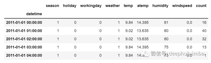
As you can see in the picture, there will be multiple columns in multivariate variables to predict the target value. (in the figure above, "count" is the target value)

In the above data, count depends not only on its previous value, but also on other characteristics. Therefore, to predict the upcoming count value, we must consider all columns including the target column to predict the target value.

One thing to remember when performing multivariate time series analysis is that we need to use multiple features to predict the current target. Let's understand it through an example-

During training, if we use 5 columns [feature1, feature2, feature3, feature4, target] to train the model, we need to provide 4 columns [feature1, feature2, feature3, feature4] for the upcoming forecast day.

LSTM

LSTM is not intended to be discussed in detail in this article. Therefore, only some simple descriptions are provided. If you don't know much about LSTM, you can refer to our previously published articles.

LSTM is basically a cyclic neural network, which can deal with long-term dependence.

Suppose you are watching a movie. So when anything happens in the film, you already know what happened before, and you can understand that new things will happen because of what happened in the past. RNNs work in the same way. They remember past information and use it to process current input. The problem with RNNs is that they cannot remember long-term dependencies because gradients disappear. Therefore, in order to avoid the problem of long-term dependence, lstm is designed.

Now we discuss time series prediction and LSTM theory. Let's start coding.

Let's first import the libraries needed for forecasting

import numpy as np
import pandas as pd
from matplotlib import pyplot as plt
from tensorflow.keras.models import Sequential
from tensorflow.keras.layers import LSTM
from tensorflow.keras.layers import Dense, Dropout
from sklearn.preprocessing import MinMaxScaler
from keras.wrappers.scikit_learn import KerasRegressor
from sklearn.model_selection import GridSearchCV

Load the data and check the output-

df=pd.read_csv("train.csv",parse_dates=["Date"],index_col=[0])
df.head()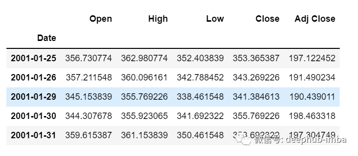

df.tail()

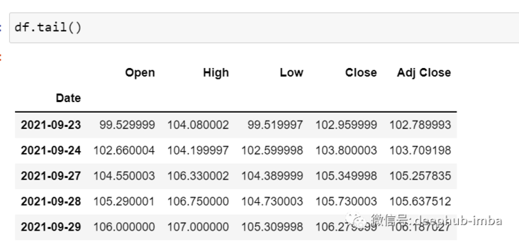
Now let's take a moment to look at the data: the csv file contains Google's stock data from 2001-01-25 to 2021-09-29. The data is based on the frequency of days.

[if you like, you can convert the frequency to "B" [business day] or "D", because we won't use the date, I just keep it as it is.]

Here we try to predict the future value of the "Open" column, so "Open" is the target column here

Let's look at the shape of the data

df.shape
(5203,5)

Now let's do the training test. We can't mess up the data here, because it must be sequential in the time series.

test_split=round(len(df)*0.20)
df_for_training=df[:-1041]
df_for_testing=df[-1041:]
print(df_for_training.shape)
print(df_for_testing.shape)

(4162, 5)
(1041, 5)

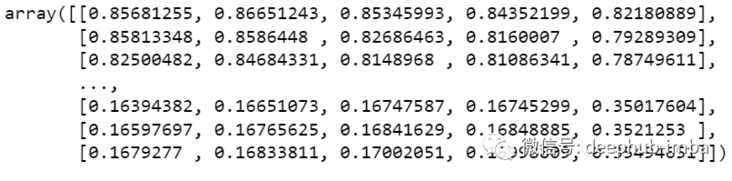
Note that the data range is very large and they are not scaled in the same range, so to avoid prediction errors, let's scale the data using MinMaxScaler first. (you can also use StandardScaler)

scaler = MinMaxScaler(feature_range=(0,1))
df_for_training_scaled = scaler.fit_transform(df_for_training)
df_for_testing_scaled=scaler.transform(df_for_testing)
df_for_training_scaled

Split the data into X and Y, which is the most important part. Read each step correctly.

def createXY(dataset,n_past):
    dataX = []
    dataY = []
    for i in range(n_past, len(dataset)):
            dataX.append(dataset[i - n_past:i, 0:dataset.shape[1]])
            dataY.append(dataset[i,0])
    return np.array(dataX),np.array(dataY)

trainX,trainY=createXY(df_for_training_scaled,30)
testX,testY=createXY(df_for_testing_scaled,30)

Let's look at what's done in the code above:

N_past is the number of steps we will look at in the past when predicting the next target value.

Using 30 here means that the past 30 values (all characteristics including the target column) will be used to predict the 31st target value.

Therefore, in trainX, we will have all eigenvalues, while in trainY, we have only target values.

Let's break down each part of the for loop

For training, dataset = df_for_training_scaled, n_past=30

When i= 30:

data_X.addend (df_for_training_scaled[i - n_past:i, 0:df_for_training.shape[1]])

From n_ The start range of past is 30, so the first data range will be - [30 - 30,30,0:5], equivalent to [0:30,0:5]

So in the dataX list, DF_ for_ training_ The scaled [0:30,0:5] array will appear for the first time.

Now, datay append(df_for_training_scaled[i,0])

i = 30, so it will only take the open starting from line 30 (because in the prediction, we only need the open column, so the column range is only 0, indicating the open column).

Storing DF in the dataY list for the first time_ for_ training_ Scaled [30,0] value.

Therefore, the first 30 rows containing 5 columns are stored in dataX, and only the 31st row of the open column is stored in dataY. Then we convert the dataX and dataY lists into arrays, which are trained in LSTM in array format.

Let's look at the shape.

print("trainX Shape-- ",trainX.shape)
print("trainY Shape-- ",trainY.shape)

(4132, 30, 5)
(4132,)

print("testX Shape-- ",testX.shape)
print("testY Shape-- ",testY.shape)

(1011, 30, 5)
(1011,)

4132 is the total number of arrays available in trainX. Each array has 30 rows and 5 columns. In trainY of each array, we have the next target value to train the model.

Let's look at one of the arrays containing (30,5) data from trainX and the trainY value of the trainX array

print("trainX[0]-- \n",trainX[0])
print("trainY[0]-- ",trainY[0])

If you look at the trainX[1] value, you will find that it is the same as the data in trainX[0] (except the first column), because we will see the first 30 to predict the 31st column. After the first prediction, it will automatically move to the second column and take the next 30 value to predict the next target value.

Let's explain all this in a simple format——

trainX — — →trainY

[0 : 30,0:5] → [30,0]

[1:31, 0:5] → [31,0]

[2:32,0:5] →[32,0]

Like this, each data will be saved in trainX and trainY

Now let's train the model. I use girdsearchCV to make some super parameter adjustments to find the basic model.

def build_model(optimizer):
    grid_model = Sequential()
    grid_model.add(LSTM(50,return_sequences=True,input_shape=(30,5)))
    grid_model.add(LSTM(50))
    grid_model.add(Dropout(0.2))
    grid_model.add(Dense(1))

grid_model.compile(loss = 'mse',optimizer = optimizer)
    return grid_modelgrid_model = KerasRegressor(build_fn=build_model,verbose=1,validation_data=(testX,testY))

parameters = {'batch_size' : [16,20],
              'epochs' : [8,10],
              'optimizer' : ['adam','Adadelta'] }

grid_search  = GridSearchCV(estimator = grid_model,
                            param_grid = parameters,
                            cv = 2)

If you want to make more superparametric adjustments for your model, you can also add more layers. However, if the data set is very large, it is recommended to add periods and units in the LSTM model.

In the first LSTM layer, the input shape is (30,5). It comes from trainx shape. (trainX.shape[1],trainX.shape[2]) → (30,5)

Now let's fit the model into trainX and trainY data.

grid_search = grid_search.fit(trainX,trainY)

This will take some time to run due to the super parameter search.

You can see that the loss will be reduced like this——

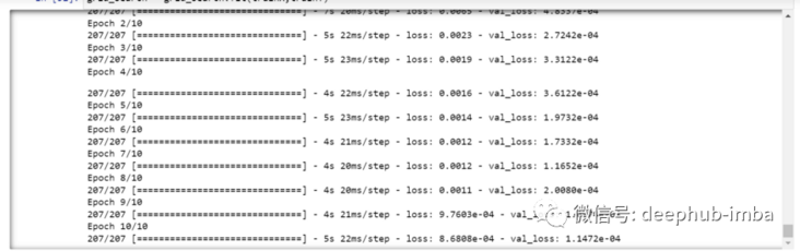
Now let's check the best parameters of the model.

grid_search.best_params_

{'batch_size': 20, 'epochs': 10, 'optimizer': 'adam'}

Save the best model in my_ In the model variable.

my_model=grid_search.best_estimator_.model

You can now test the model with the test dataset.

prediction=my_model.predict(testX)
print("prediction\n", prediction)
print("\nPrediction Shape-",prediction.shape)

The length of test and prediction are the same. You can now compare testY with the forecast.

But we scaled the data at the beginning, so first we must do some inverse scaling process.

scaler.inverse_transform(prediction)

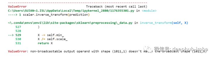
An error is reported. This is because when scaling data, we have 5 columns per row. Now we only have 1 column as the target column.

So we have to change the shape to use inverse_transform

prediction_copies_array = np.repeat(prediction,5, axis=-1)

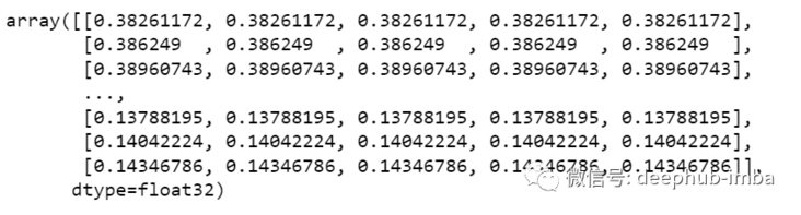
The 5 column values are similar, except that a single forecast column is copied 4 times. So now we have five columns of the same value.

prediction_copies_array.shape
(1011,5)

This allows you to use inverse_transform function.

pred=scaler.inverse_transform(np.reshape(prediction_copies_array,(len(prediction),5)))[:,0]

But the first column after inverse transformation is what we need, so we use → [:, 0] at the end.

Now compare the pred value with testY, but testY is also scaled, and you also need to use the same code as above for inverse transformation.

original_copies_array = np.repeat(testY,5, axis=-1)
original=scaler.inverse_transform(np.reshape(original_copies_array,(len(testY),5)))[:,0]

Now let's look at the predicted value and the original value →

print("Pred Values-- " ,pred)
print("\nOriginal Values-- " ,original)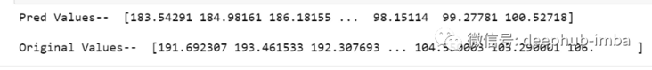

Finally, draw a graph to compare our pred with the original data.

plt.plot(original, color = 'red', label = 'Real Stock Price')
plt.plot(pred, color = 'blue', label = 'Predicted Stock Price')
plt.title('Stock Price Prediction')
plt.xlabel('Time')
plt.ylabel('Google Stock Price')
plt.legend()
plt.show()

It looks good. So far, we have trained the model and checked the model with test values. Now let's predict some future values.

Get the last 30 values we loaded at the beginning from the main df dataset [why 30? Because this is the number of past values we want to predict the 31st value]

df_30_days_past=df.iloc[-30:,:]
df_30_days_past.tail()

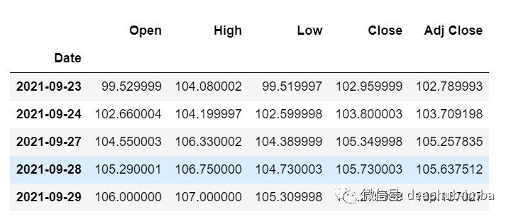
You can see that there are all columns including the target column ("Open"). Now let's predict the next 30 values.

In multivariate time series prediction, we need to use different features to predict a single column, so we need to use eigenvalues (except target columns) to predict the coming.

Here, we need the upcoming 30 values of "High", "Low", "Close" and "Adj Close" columns to predict the "Open" column.

df_30_days_future=pd.read_csv("test.csv",parse_dates=["Date"],index_col=[0])
df_30_days_future

After the "Open" column is eliminated, the following operations need to be done before using the model for prediction:

Scale the data because the 'Open' column is deleted. Before scaling it, add an Open column with all values of "0".

After scaling, replace the "Open" column value in the future data with "nan"

Now append the 30 day old value and the 30 day new value (where the last 30 open values are nan)

df_30_days_future["Open"]=0
df_30_days_future=df_30_days_future[["Open","High","Low","Close","Adj Close"]]
old_scaled_array=scaler.transform(df_30_days_past)
new_scaled_array=scaler.transform(df_30_days_future)
new_scaled_df=pd.DataFrame(new_scaled_array)
new_scaled_df.iloc[:,0]=np.nan
full_df=pd.concat([pd.DataFrame(old_scaled_array),new_scaled_df]).reset_index().drop(["index"],axis=1)

full_ The DF shape is (60,5), and the last first column has 30 nan values.

To make a prediction, we must use the for loop again, what we did when we split the data in trainX and trainY. But this time we only have X, not Y

full_df_scaled_array=full_df.values
all_data=[]
time_step=30
for i in range(time_step,len(full_df_scaled_array)):
    data_x=[]
    data_x.append(
     full_df_scaled_array[i-time_step :i , 0:full_df_scaled_array.shape[1]])
    data_x=np.array(data_x)
    prediction=my_model.predict(data_x)
    all_data.append(prediction)
    full_df.iloc[i,0]=prediction

For the first prediction, there are the first 30 values. When the for loop runs for the first time, it checks the first 30 values and predicts the 31st "Open" data.

When the second for loop will try to run, it will skip the first line and try to get the next 30 values [1:31]. An error will be reported here because the last row of the Open column is "nan", so you need to replace "nan" with a forecast every time.

Finally, the inverse transformation →

new_array=np.array(all_data)
new_array=new_array.reshape(-1,1)
prediction_copies_array = np.repeat(new_array,5, axis=-1)
y_pred_future_30_days = scaler.inverse_transform(np.reshape(prediction_copies_array,(len(new_array),5)))[:,0]
print(y_pred_future_30_days)

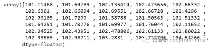
Such a complete process has run through.

If you want to see the complete code, you can view it here:

https://www.overfit.cn/post/1...

Author: Sksujanislam