Neural network foundation and multi class classification
3.1 model representation
3.1.1 why do we need neural networks
Both linear regression and logistic regression learned in the first two sections have a disadvantage: when there are too many features, the calculation load will be very large. For example, in identifying whether a picture is a car, we regard the pixels of the picture as features. If we also need to combine features to form a polynomial model, there may be millions of features, so we need neural network.
3.1.2 neuron and neural network model
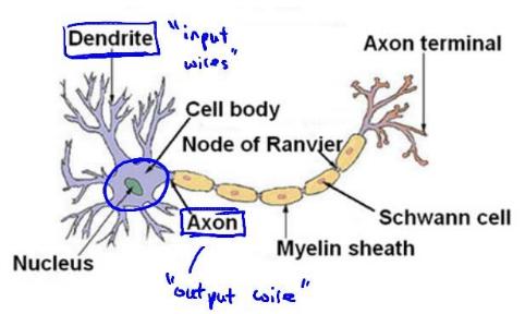
The above figure is a schematic diagram of a neuron. Each neuron can be considered as a processing unit / nucleus, which contains many input / dendrites and has an output / axon.
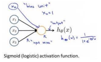
Neural network model is based on many neurons, and each neuron is a learning model. These neurons take features as inputs and provide an output according to the neuron model. The following figure is an example of a neuron, using a logistic regression model as its own learning model.
In neural networks, parameters
θ
\theta
θ Also known as weight
Neural network model is a network organized by many neurons according to different levels. The output variables of each layer are the input variables of the next layer. The following figure shows a three-layer neural network.
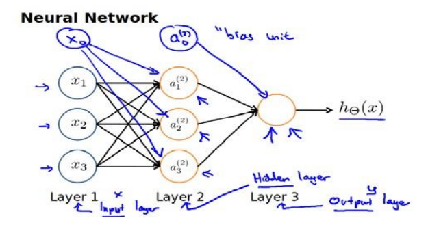
The first layer is the input layer, where
x
1
,
x
2
,
x
3
x_1,x_2,x_3
x1, x2, x3 are input units to which we input raw data. The last layer is the output layer, in which the neuron is called the output unit, which is responsible for calculation
h
θ
(
x
)
h_\theta(x)
h θ (x). The middle layer is called the hidden layer,
a
1
,
a
2
,
a
3
a_1,a_2,a_3
a1, a2 and a3 are intermediate units, which are responsible for processing data and become more "advanced" features. Introduced in the previous two sections
x
0
=
1
x_0=1
x0 = 1, a bias unit is added in the non output layer of the neural network
We introduce tagging to help us understand the model:
a
i
(
j
)
a_i^{(j)}
ai(j) stands for the third party
j
j
Layer j
i
i
i activation units.
Θ
(
j
)
\Theta^{(j)}
Θ (j) Representative from No
j
j
Layer j is mapped to the second layer
j
+
1
j+1
For the weight matrix of layer j+1, the number of rows is the number of active units of the next layer, and the number of columns is the number of active units of the current layer plus one (because offset units are added), as shown in the above figure
Θ
(
1
)
\Theta^{(1)}
Θ (1) The size of the is
3
×
4
3\times4
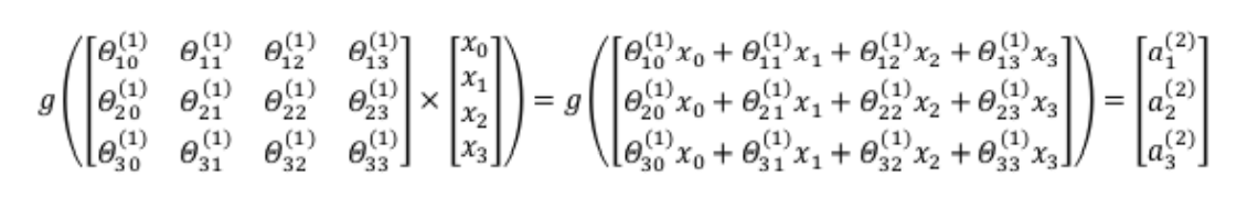
three × 4. The activation unit and output in the figure above are respectively expressed as:
a
1
(
2
)
=
g
(
θ
10
(
1
)
x
0
+
θ
11
(
1
)
x
1
+
θ
12
(
1
)
x
2
+
θ
13
(
1
)
x
3
)
a
2
(
2
)
=
g
(
θ
20
(
1
)
x
0
+
θ
21
(
1
)
x
1
+
θ
22
(
1
)
x
2
+
θ
23
(
1
)
x
3
)
a
3
(
2
)
=
g
(
θ
30
(
1
)
x
0
+
θ
31
(
1
)
x
1
+
θ
32
(
1
)
x
2
+
θ
33
(
1
)
x
3
)
h
θ
(
x
)
=
g
(
θ
10
(
2
)
a
0
+
θ
11
(
1
)
a
1
+
θ
12
(
2
)
a
2
+
θ
13
(
2
)
a
3
)
\begin{aligned} a_1^{(2)}=g(\theta_{10}^{(1)}x_0+\theta_{11}^{(1)}x_1+\theta_{12}^{(1)}x_2+\theta_{13}^{(1)}x_3)\\ a_2^{(2)}=g(\theta_{20}^{(1)}x_0+\theta_{21}^{(1)}x_1+\theta_{22}^{(1)}x_2+\theta_{23}^{(1)}x_3)\\ a_3^{(2)}=g(\theta_{30}^{(1)}x_0+\theta_{31}^{(1)}x_1+\theta_{32}^{(1)}x_2+\theta_{33}^{(1)}x_3)\\ h_\theta(x)=g(\theta_{10}^{(2)}a_0+\theta_{11}^{(1)}a_1+\theta_{12}^{(2)}a_2+\theta_{13}^{(2)}a_3) \end{aligned}
a1(2)=g(θ10(1)x0+θ11(1)x1+θ12(1)x2+θ13(1)x3)a2(2)=g(θ20(1)x0+θ21(1)x1+θ22(1)x2+θ23(1)x3)a3(2)=g(θ30(1)x0+θ31(1)x1+θ32(1)x2+θ33(1)x3)hθ(x)=g(θ10(2)a0+θ11(1)a1+θ12(2)a2+θ13(2)a3)
The above discussion only feeds one row of the characteristic matrix (a training example) to the neural network. We need to feed the whole data set to our neural network to learn the model. From the expression, we can get each
a
a
a is all from the upper layer
x
x
x and the corresponding weight. We call this algorithm from left to right forward propagation algorithm
Compared with cyclic coding, the forward propagation algorithm is simpler to use vectorization. Take the above figure as an example to calculate the value of the second layer activation unit.
X
=
[
x
0
x
1
x
2
x
3
]
z
(
2
)
=
[
z
1
(
2
)
z
2
(
2
)
z
3
(
3
)
]
{\begin{matrix} X=\begin{bmatrix} x_0 \\ x_1 \\ x_2 \\ x_3 \end{bmatrix} & z^{(2)} =\begin{bmatrix} z_1^{(2)}\\ z_2^{(2)}\\ z_3^{(3)} \end{bmatrix} \end{matrix}}
X=⎣⎢⎢⎡x0x1x2x3⎦⎥⎥⎤z(2)=⎣⎢⎡z1(2)z2(2)z3(3)⎦⎥⎤
z
(
2
)
=
Θ
(
1
)
x
a
(
2
)
=
g
(
z
(
2
)
)
z^{(2)}=\Theta^{(1)}x\\ a^{(2)}=g(z^{(2)})
z(2)=Θ(1)xa(2)=g(z(2))
order
z
(
2
)
=
Θ
(
1
)
x
z^{(2)}=\Theta^{(1)}x
z(2)= Θ (1)x, then
a
(
2
)
=
g
(
z
(
2
)
)
a^{(2)}=g(z^{(2)})
a(2)=g(z(2)), added after calculation
a
0
(
2
)
=
1
a_0^{(2)}=1
a0(2)=1. After calculation, the output value is:
We order
z
(
3
)
=
Θ
(
2
)
a
(
2
)
z^{(3)}=\Theta^{(2)}a^{(2)}
z(3)= Θ (2)a(2), then
h
θ
(
x
)
=
a
(
3
)
=
g
(
z
(
3
)
)
h_\theta(x)=a^{(3)}=g(z^{(3)})
hθ(x)=a(3)=g(z(3)).
The above discussion is only the calculation of a training example. If we want to calculate the whole training set, we need to transpose the feature matrix of the training set so that the features of the same training instance are in the same column. Namely:
z
(
2
)
=
Θ
(
1
)
×
X
T
a
(
2
)
=
g
(
z
(
2
)
)
z^{(2)}=\Theta^{(1)}\times X^T\\ a^{(2)}=g(z^{(2)})
z(2)=Θ(1)×XTa(2)=g(z(2))
From the above expression, we can see that the neural network based on sigmoid is like Logistic regression. We can regard the activation units of the middle layer as higher-level eigenvalues, which are composed of
x
x
x decision can better predict new data.
3.2 intuitive understanding of the model
3.2.1 monolayer neurons
In the neural network, the prediction made by the output layer uses the features in the hidden layer rather than the original features of the input layer. We can think that the features in the second layer are a series of new features obtained by the neural network after learning to predict the output variables.
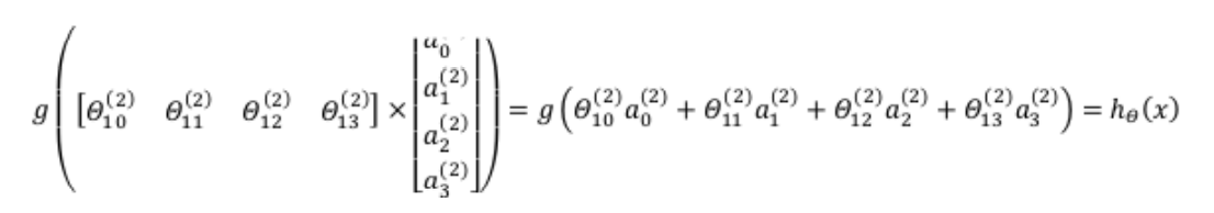
We use a single-layer neuron to represent logical operations, such as logical and, logical or.
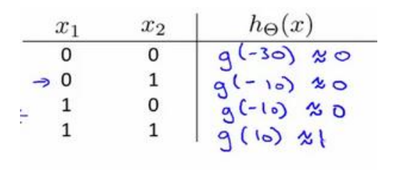
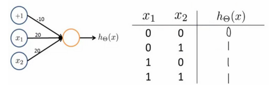
Example: logical AND (AND)
among
θ
0
=
−
30
,
θ
1
=
20
,
θ
2
=
20
\theta_0=-30,\theta_1=20,\theta_2=20
θ 0=−30, θ 1=20, θ 2 = 20, the output function is
h
θ
(
x
)
=
g
(
−
30
+
20
x
1
+
20
x
2
)
.
h_\theta(x)=g(-30+20x_1+20x_2).
hθ(x)=g(−30+20x1+20x2).
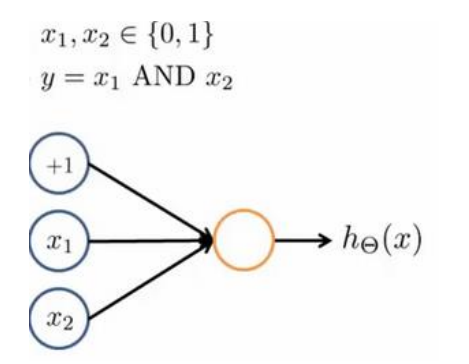
We know that the image of sigmoid function is:
z
=
4.6
z=4.6
When z=4.6,
g
(
z
)
≈
0.99
g(z)\approx0.99
g(z)≈0.99;
z
=
−
4.6
z=-4.6
When z = − 4.6,
g
(
z
)
≈
0.01
g(z)\approx0.01
g(z)≈0.01
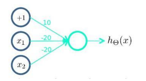
Similarly, the OR function can be expressed as follows:
( N O T x 1 ) A N D ( N O T x 2 ) (NOTx_1)AND(NOTx_2) (NOTx1) AND(NOTx2) functions (or non functions) can be expressed as follows:
3.2.2 neuron combination
When we want to achieve
X
N
O
R
XNOR
XNOR (same or) function,
X
N
O
R
=
(
x
1
A
N
D
x
2
)
O
R
(
(
N
O
T
x
1
)
A
N
D
(
N
O
T
x
2
)
)
XNOR=(x_1 AND x_2)OR((NOT x_1)AND(NOTx_2))
XNOR=(x1ANDx2)OR((NOTx1)AND(NOTx2))
Thus, we can combine single-layer neurons to obtain the functional expression to realize more complex functions.
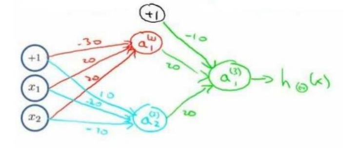
Among them,
a
1
(
2
)
a_1^{(2)}
a1(2) realizes
x
1
And
x
2
x_1 and X_ two
The sum of x1 and x2,
a
2
(
2
)
a_2^{(2)}
a2(2) realizes
x
1
And
x
2
x_1 and X_ two
The or non operation of x1 and x2,
a
1
(
3
)
a_1^{(3)}
a1(3) realizes
a
1
(
2
)
And
a
2
(
2
)
a_1^{(2)} and a_2^{(2)}
The or operation of a1(2) and a2(2).
In this way, we can gradually construct more and more complex functions and get stronger characteristics.
3.3 multi category classification
When we have more than two categories, such as identifying passers-by, cars, motorcycles and trucks through pictures, the output layer should have four values.
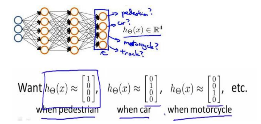
The output result of neural network algorithm is one of four possible cases:
[
1
0
0
0
]
[
0
1
0
0
]
[
0
0
1
0
]
[
0
0
0
1
]
\begin{matrix} \begin{bmatrix} 1\\ 0\\ 0\\ 0 \end{bmatrix} \begin{bmatrix} 0\\ 1\\ 0\\ 0 \end{bmatrix} \begin{bmatrix} 0\\ 0\\ 1\\ 0 \end{bmatrix} \begin{bmatrix} 0\\ 0\\ 0\\ 1 \end{bmatrix} \end{matrix}
⎣⎢⎢⎡1000⎦⎥⎥⎤⎣⎢⎢⎡0100⎦⎥⎥⎤⎣⎢⎢⎡0010⎦⎥⎥⎤⎣⎢⎢⎡0001⎦⎥⎥⎤
3.4 Python implementation of supporting operations
3.4.1 logistic expression realizes multi class classification
1. Problem background
You will use logistic regression and neural networks to recognize handwritten digits (from 0 to 9).
Automatic handwritten numeral recognition is widely used today: from recognizing postal code (postal code) to recognizing the amount on bank check on mail envelope. This exercise will show you how the methods you have learned can be used for this classification task.
2. Code implementation
Let's import the library we need first.
import matplotlib.pyplot as plt
import numpy as np
import scipy.io as sio
import matplotlib
import scipy.optimize as opt
from sklearn.metrics import classification_report#This package is an evaluation report
Import the data set. The data set given by Wu Enda is a mat file and needs to use SciPy IO to load data.
At the same time, the given data set is (5000400), and 400 is 20 × 20 gray value, 5000 training examples. But we need to put 20 × 20 transpose to get the picture in the correct direction.
def load_data(path, transpose=True):
    data = sio.loadmat(path)
    y = data.get('y')  # (5000,1)
    y = y.reshape(y.shape[0])  # make it back to column vector

    X = data.get('X')  # (5000,400)

    if transpose:
        # for this dataset, you need a transpose to get the orientation right
        X = np.array([im.reshape((20, 20)).T for im in X])

        # and I flat the image again to preserve the vector presentation
        X = np.array([im.reshape(400) for im in X])

    return X, y


X, y = load_data('ex3data1.mat')
print(X.shape)
print(y.shape)
We can draw pictures through data sets to deepen our understanding of gray values and data sets.
def plot_an_image(image):
    """
    image : (400,)
    """
    fig, ax = plt.subplots(figsize=(1, 1))
    ax.matshow(image.reshape((20, 20)), cmap=matplotlib.cm.binary)
    plt.xticks(np.array([]))  # just get rid of ticks
    plt.yticks(np.array([]))


pick_one = np.random.randint(0, 5000)
plot_an_image(X[pick_one, :])
plt.show()
print('this should be {}'.format(y[pick_one]))
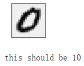
Note that the y value of 0 in this dataset is 10
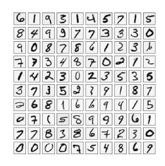
def plot_100_image(X):
    """ sample 100 image and show them
    assume the image is square

    X : (5000, 400)
    """
    size = int(np.sqrt(X.shape[1]))

    # sample 100 image, reshape, reorg it
    sample_idx = np.random.choice(np.arange(X.shape[0]), 100)  # 100*400
    sample_images = X[sample_idx, :]

    fig, ax_array = plt.subplots(nrows=10, ncols=10, sharey=True, sharex=True, figsize=(8, 8))

    for r in range(10):
        for c in range(10):
            ax_array[r, c].matshow(sample_images[10 * r + c].reshape((size, size)),
                                   cmap=matplotlib.cm.binary)
            plt.xticks(np.array([]))
            plt.yticks(np.array([]))
            #Drawing function, draw 100 pictures


plot_100_image(X)
plt.show()
raw_X, raw_y = load_data('ex3data1.mat')
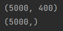
print(raw_X.shape)
print(raw_y.shape)
(5000, 400)
(5000,)
First, we sort out the data. We need to insert a column of 1 before X as the offset unit.
# add intercept=1 for x0
X = np.insert(raw_X, 0, values=np.ones(raw_X.shape[0]), axis=1)#First column inserted (all 1)
X.shape
(5000, 401)
For y we do vectorization label processing, and the final dimension is 10 × 5000, each line represents the relationship with the number. For example, the first line, y[0] represents whether the sample is 0 (because I put line 10 in the first line) by analogy, we get the binary prediction of each number (yes or no), and finally get the output vector.
# y have 10 categories here. 1..10, they represent digit 0 as category 10 because matlab index start at 1
# I'll ditit 0, index 0 again
y_matrix = []

for k in range(1, 11):
    y_matrix.append((raw_y == k).astype(int))  # See the figure "vectorization label. png"

# last one is k==10, it's digit 0, bring it to the first position, the last line k=10, all 0, put the last line to the first line
y_matrix = [y_matrix[-1]] + y_matrix[:-1]
y = np.array(y_matrix)

print(y.shape)

# Expand 5000 to 10 * 5000
#     For example, y = 10 - > [0, 0, 0, 0, 0, 0, 0, 0, 0, 1]: ndarray is a single column
We start with training one-dimensional model, that is, we use logistic regression to realize binary classification, such as judging whether the number is 0 We can directly use the cost function and gradient function written in the previous section.
"""
Matrix calculation method for calculating cost function and gradient
matrix *Matrix multiplication
array @Matrix multiplication *Multiply corresponding elements
def cost(theta, X, y, l=1):
    # INPUT: parameter value theta, data X, tag y, learning rate
    # OUTPUT: cross entropy loss under current parameter value
    # TODO: calculate the cross entropy loss function according to the parameters and input data

    # STEP1: convert theta, X, y to a matrix of type numpy
    theta = np.matrix(theta)
    X = np.matrix(X)
    y = np.matrix(y)

    # STEP2: calculate the loss function according to the formula (excluding regularization)

    cross_cost = np.mean(np.multiply(y, np.log(sigmoid(X * theta.T))) - np.multiply((1 - y), np.log(1 - sigmoid(X * theta.T))))

    # STEP3: calculate the regularization part of the loss function according to the formula
    reg = (l / (2 * len(X))) * np.power(theta[1:], 2).sum()

    # STEP4: add up the results in the previous two steps to obtain the overall loss function
    whole_cost = cross_cost + reg

    return whole_cost


def sigmoid(z):
    return 1 / (1 + np.exp(-z))


def gradient(theta, X, y, l=1):
    theta = np.matrix(theta)
    X = np.matrix(X)
    y = np.matrix(y).T

    parameters = int(theta.ravel().shape[1])
    error = sigmoid(X * theta.T) - y
    grad = ((X.T * error) / len(X)).T + ((l / len(X)) * theta)

    # intercept gradient is not regularized
    grad[0, 0] = np.sum(np.multiply(error, X[:, 0])) / len(X)

    return np.array(grad).ravel()
"""


def sigmoid(z):
    return 1 / (1 + np.exp(-z))


def cost(theta, X, y, l=1):
    ''' cost fn is -l(theta) for you to minimize'''
    return np.mean(-y * np.log(sigmoid(X @ theta)) - (1 - y) * np.log(1 - sigmoid(X @ theta)))


def regularized_cost(theta, X, y, l=1):
    '''you don't penalize theta_0'''
    theta_j1_to_n = theta[1:]
    regularized_term = (l / (2 * len(X))) * np.power(theta_j1_to_n, 2).sum()

    return cost(theta, X, y) + regularized_term


def regularized_gradient(theta, X, y, l=1):
    '''still, leave theta_0 alone'''
    theta_j1_to_n = theta[1:]
    regularized_theta = (l / len(X)) * theta_j1_to_n

    # by doing this, no offset is on theta_0
    regularized_term = np.concatenate([np.array([0]), regularized_theta])

    return gradient(theta, X, y) + regularized_term


def gradient(theta, X, y, l=1):
    '''just 1 batch gradient'''
    return (1 / len(X)) * X.T @ (sigmoid(X @ theta) - y)


def logistic_regression(X, y, l=1):
    """generalized logistic regression
    args:
        X: feature matrix, (m, n+1) # with incercept x0=1
        y: target vector, (m, )
        l: lambda constant for regularization

    return: trained parameters
    """
    # init theta
    theta = np.zeros(X.shape[1])

    # train it
    res = opt.minimize(fun=regularized_cost,
                       x0=theta,
                       args=(X, y, l),
                       method='TNC',
                       jac=regularized_gradient,
                       options={'disp': True}
                       )
    # get trained parameters
    final_theta = res.x

    return final_theta


def predict(x, theta):
    prob = sigmoid(x @ theta)
    return (prob >= 0.5).astype(int)


t0 = logistic_regression(X, y[0])
print(t0.shape)
y_pred = predict(X, t0)
print('Accuracy={}'.format(np.mean(y[0] == y_pred)))
(401,)
Accuracy=0.9974
Next, we train the k-dimensional model and generate the output vector to get the classification results.
k_theta = np.array([logistic_regression(X, y[k]) for k in range(10)])
print(k_theta.shape)
(10, 401)
Now let's consider the dimension problem of k-dimensional model in prediction
X
×
θ
T
X\times \theta^T
X×θT.
(
5000
,
401
)
×
(
10
,
401
)
T
=
(
5000
,
10
)
(5000,401)×(10,401)^T=(5000,10)
(5000,401)×(10,401)T=(5000,10)
Therefore, the output vector of each sample of each behavior of the final result can identify the number.
prob_matrix = sigmoid(X @ k_theta.T)
# np.set_printoptions(suppress=True) the scientific counting method is not used for large / small numbers
y_pred = np.argmax(prob_matrix, axis=1)  # Returns the index of the maximum value along the axis, where axis=1 represents the row

y_answer = raw_y.copy()  # Correct result
y_answer[y_answer==10] = 0
print(classification_report(y_answer, y_pred))
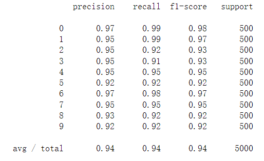
3.4.2 prediction of forward propagation algorithm
1. Problem background
Same as 3.4.1
2. Model display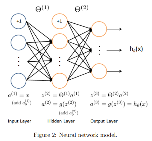
3. Code implementation
def load_weight(path):
    data = sio.loadmat(path)
    return data['Theta1'], data['Theta2']
theta1, theta2 = load_weight('ex3weights.mat')

theta1.shape, theta2.shape
((25, 401), (10, 26))
It can be seen that the number of neurons in the middle layer is 25 and the bias unit is 26
Because in the data loading function, the original data is transposed. However, the transposed data is incompatible with the given parameters because these parameters are trained by the original data. So in order to apply the given parameters, I need to use the raw data (no transpose).
X, y = load_data('ex3data1.mat',transpose=False)

X = np.insert(X, 0, values=np.ones(X.shape[0]), axis=1)  # intercept

X.shape, y.shape
((5000, 401), (5000,))
Once the data is ready, you can start feed forward prediction
a1 = X
z2 = X @ theta1.T # (5000, 401) @ (25,401).T = (5000, 25)
a2 = sigmoid(z2)
a2 = np.insert(a2, 0, values=np.ones(a2.shape[0]), axis=1)
z3 = a2 @ theta2.T
a3 = sigmoid(z3)

y_pred = np.argmax(a3, axis=1) + 1  # numpy is 0 base index, +1 for matlab convention, returns the index of the maximum value along axis, axis=1 represents the row
The output vector is 1, 2,..., 10 (0) in turn. In python, the subscript starts from 0, so you need to + 1 in the result
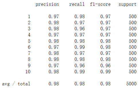
print(classification_report(y, y_pred))