Non ranging location algorithm

This kind of localization algorithm estimates the target by relying on the physical deployment of the observation station and the simple binary detection information of "yes" and "no" of the detected target. There are mainly centroid localization algorithm, weighted centroid localization algorithm and network localization algorithm.

1. Centroid location algorithm

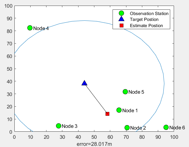
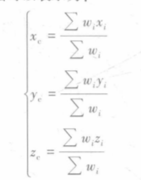
For multi particle system, the position of each particle is p(xi,yi,zi). Considering that the mass of each particle is the same, the calculation method of centroid is as follows:

Taking the position of the observation station as the position of the particle, the estimated value of the target position can be calculated according to the above formula. When the observation stations are sparse step by step, the positioning error will be large.

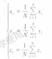
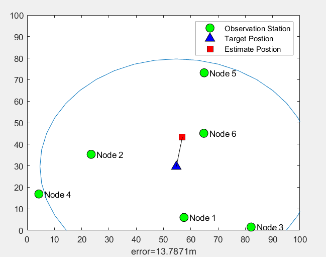
Example: suppose that there are 6 observation stations randomly deployed on the site with length and width of 100m, each observation station is exactly the same, and the detection distance is 50m. A target appears randomly in the site, is observed by the observation station, and the estimated position is calculated. Matlab simulation is as follows:

function CentroidLocalization        %Centroid location algorithm
%Positioning initialization
Length=100;                          %Site space in meters
Width=100;                           %Site space in meters
d=50;                                %Observation station detection capacity 50 m
N=6;                                 %Number of observation stations
for i=1:N                            %Position initialization of observation station
    Node(i).x=Width*rand;
    Node(i).y=Length*rand;    
end
%The real location of the target is also given randomly here
Target.x=Width*rand;
Target.y=Length*rand;  
X=[ ];                               %Used to save the location of the detection station where the target is detected
for i=1:N
    if getDist(Node(i),Target)<=d    %Call the distance function, getDist()Function must be written in another m In the document, see the end
        X=[X;Node(i).x, Node(i).y];  %Save the location of the detection station where the target is detected
    end
end
M=size(X,1);                         %Number of observation stations detecting targets
if M>0
    Est_Target.x=sum(X(:,1))/M;      %Estimated position of centroid x
    Est_Target.y=sum(X(:,2))/M;      %Estimated position of centroid y
    Error_Dist=getDist(Est_Target,Target)     %Error between estimated and actual centroid values
end
%Start drawing
figure
hold on;box on;axis([0 100 0 100]);
for i=1:N
	h1=plot(Node(i).x,Node(i).y,'ko','MarkerFace','g','MarkerSize',10);
    text(Node(i).x+2,Node(i).y,['Node ',num2str(i)]);   
end
%Draw the real position and estimated position of the target
h2=plot(Target.x,Target.y,'k^','MarkerFace','b','MarkerSize',10);   %Draw the real position
h3=plot(Est_Target.x,Est_Target.y,'ks','MarkerFace','r','MarkerSize',10);   %Draw the estimated position
%Connect the real position of the target with the estimated position with a line
line ([Target.x,Est_Target.x],[Target.y,Est_Target.y],'Color','k');   
%Draw around the target to detect capability 50 m Circle with radius d Range; circle()Function written in circle.m In the file
circle(Target.x,Target.y,d);  
%indicate h1,h2,h3 What is it?
legend([h1,h2,h3],'Observation Station','Target Postion','Estimate Postion');
xlabel(['error=',num2str(Error_Dist),'m']);

%To calculate the two-point distance function, you must write it in another m In the file
function dist=getDist(A,B)
dist=sqrt((A.x-B.x)^2+(A.y-B.y)^2);
end

%To draw a circle function, you must write it in another m In the file
function circle(x0,y0,r)
sita=0:pi/20:2*pi;
plot (x0+r*cos(sita),y0+r*sin(sita));
end

Operation results:


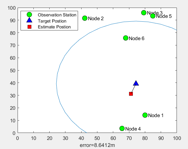
The two operation results show that the errors are 8.6m and 28.0m respectively. The two positioning errors are very different. The positioning error is closely related to the position and deployment density of the observation station.

2. Weighted centroid location algorithm

When detecting a target, the sensor can roughly judge the distance of the target according to the strength of the detected target signal, such as sound signal strength or wireless received signal strength (RSSI), and use this strength as a weight in the centroid positioning algorithm:

Generally, the weight has a certain proportional relationship with the distance. For example, RSSI has an inverse relationship with the approximate distance. During modeling, it can be roughly considered that:

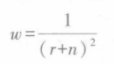
Note: r is the distance between the target and the observation station; n is noise, indicating that the strength of RSSI and sound signals measured by the observation station are disturbed by noise. For the given method of noise size, refer to the Signal to Noise Ratio (SNR) parameter:

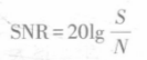
Note: S represents the signal value, and here represents the received signal strength value; N represents the variance of noise. If the signal-to-noise ratio is 10dB, then N = S / 2 N=S/ \sqrt{2} \quad N=S/2 ​

For example, six observation stations are randomly deployed on a 100m*100m site. The detection distance of each observation station is 50m, and the strength of the sound signal from the target to the observation station can be detected. The observation station detects the targets in the site, and MATLAB simulation:

function WeightCentroidLocalization        %Weighted centroid location algorithm
%Positioning initialization
Length=100;                          %Site space in meters
Width=100;                           %Site space in meters
d=50;                                %Observation station detection capacity 50 m
Node_number=6;                       %Number of observation stations
SNR=50;                              %Signal to noise ratio
for i=1:Node_number                  %Position initialization of observation station
    Node(i).x=Width*rand;
    Node(i).y=Length*rand;    
end
%The real location of the target is also given randomly here
Target.x=Width*rand;
Target.y=Length*rand;  
%Observation station detection target
X=[ ];W=[ ];                         %Weight 
for i=1:Node_number
	dd=getdist(Node(i),Target);
	Q=dd/(10^(20/SNR));              %Calculate the noise variance according to the signal-to-noise ratio formula
    if dd<=d
        X=[X;Node(i).x, Node(i).y]; 
        W=[W,1/((dd+sqrt(Q)*randn)^2)]; %Calculate the weight according to the formula
    end
end
%Weight normalization
W=W./sum(W);
N=size(X,1);                         %Number of observation stations detecting targets
sumx=0;sumy=9;
for i=1:N
	sumx=sumx+X(i,1)*W(i);
	sumy=sumy+X(i,2)*W(i);
end
Est_Target.x=sumx;      %Estimated location of target x
Est_Target.y=sumy;      %Target estimated location y
Error_Dist=getdist(Est_Target,Target)     %Error between target estimated value and actual value

%Start drawing
figure
hold on;box on;axis([0 100 0 100]);
for i=1:Node_number
	h1=plot(Node(i).x,Node(i).y,'ko','MarkerFace','g','MarkerSize',10);
    text(Node(i).x+2,Node(i).y,['Node ',num2str(i)]);   
end
%Draw the real position and estimated position of the target
h2=plot(Target.x,Target.y,'k^','MarkerFace','b','MarkerSize',10);   %Draw the real position
h3=plot(Est_Target.x,Est_Target.y,'ks','MarkerFace','r','MarkerSize',10);   %Draw the estimated position
%Connect the real position of the target with the estimated position with a line
line ([Target.x,Est_Target.x],[Target.y,Est_Target.y],'Color','k');   
%Draw around the target to detect capability 50 m Circle with radius d Range; circle()Function written in circle.m In the file
circle(Target.x,Target.y,d);  
%indicate h1,h2,h3 What is it?
legend([h1,h2,h3],'Observation Station','Target Postion','Estimate Postion');
xlabel(['error=',num2str(Error_Dist),'m']);

%To calculate the two-point distance function, you must write it in another m In the file
function dist=getdist(A,B)
dist=sqrt((A.x-B.x)^2+(A.y-B.y)^2);
end

%To draw a circle function, you must write it in another m In the file
function circle(x0,y0,r)
sita=0:pi/20:2*pi;
plot (x0+r*cos(sita),y0+r*sin(sita));
end

Operation results:

3. Grid location algorithm

The grid positioning algorithm is that the observation stations are uniformly deployed in the detection site and arranged in the form of queue grid.

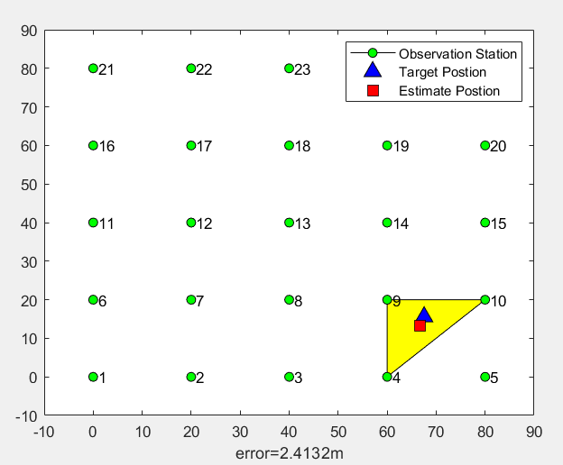
Example: suppose the target is in a 100m*100m site, an observation station is placed every 20m, and the detection distance of the observation station is 50m. When multiple observation stations detect the target, the centroid of the position of the three base stations with the strongest target signal is used as the estimated position of the target. The MATLAB simulation is as follows:

function CridLocalization            %Grid location algorithm
%Positioning initialization
Length=100;                          %Site space in meters
Width=100;                           %Site space in meters
Xnum=5;                              %Number of observation stations in horizontal direction
Ynum=5;                              %Number of observation stations in vertical direction
divX=Length/Xnum/2;divY=Width/Ynum/2;%In order to view the station step-by-step adjustment in the middle
d=50;                                %Observation station detection capacity 50 m
Target.x=Width * (Xnum-1)/Xnum * rand;
Target.y=Length * (Ynum-1)/Ynum * rand;
DIST=[ ];                            %Place a collection of distances between the observation station and the target
for j=1:Ynum                         %Grid deployment of observation stations
    for i=1:Xnum
        Station((j-1) * Xnum+i).x=(i-1) * Length/Xnum;
        Station((j-1) * Xnum+i).y=(j-1) * Width/Ynum;
        dd=getdist(Station((j-1) * Xnum+i) ,Target);
        DIST=[DIST dd];
    end
end
%Find out the three observation stations with the strongest detected target signal, that is, the observation station closest to the target
[set,index] =sort( DIST);             % set Is an ordered set of values from small to large, index Is an indexed collection
NI=index(1:3);                        %Last 3,Namely index 1-3 Elements
Est_Target.x=0;Est_Target.y=0;
if set(NI(3))<d                       %Check whether the largest of the three is within the detectable range of the observation station
    for i=1:3
        Est_Target.x= Est_Target.x+Station(NI(i)).x/3;
        Est_Target.y= Est_Target.y+Station(NI(i)).y/3;
    end
end

%Start drawing
figure
hold on;box on;axis([0-divX,Length-divX,0-divY,Width-divX])
xx=[Station(NI(1)).x,Station(NI(2)).x,Station(NI(3)).x];
yy=[Station( NI(1)).y,Station( NI(2)).y,Station(NI(3)).y];
fill(xx,yy,'y');
for j=1:Ynum
    for i=1:Xnum
        h1=plot(Station((j-1) * Xnum+i).x,Station((j-1) * Xnum+i).y,'-ko','MarkerFace','g');
        text(Station((j-1) * Xnum+i).x+1,Station((j-1) * Xnum+i).y, num2str((j-1) * Xnum+i));
    end
end
Error_Est=getdist( Est_Target,Target)
h2=plot(Target.x,Target.y,'k^','MarkerFace','b' ,'MarkerSize', 10) ;
h3=plot(Est_Target.x,Est_Target.y,'ks','MarkerFace','r','MarkerSize',10);
legend([h1,h2,h3] ,'Observation Station', 'Target Postion' ,'Estimate Postion');
xlabel(['error=',num2str(Error_Est),'m']);

%To calculate the two-point distance function, you must write it in another m In the file
function dist=getdist(A,B)
dist=sqrt((A.x-B.x)^2+(A.y-B.y)^2);
end

Operation results: