reference material:

[1] (this PPT is very popular, but a knowledge point is omitted for the content of multi interpolation point piecewise curve) Algorithm of cubic periodic B-spline curve - Baidu Library (baidu.com)

[2] (this introduces the cubic B-spline curve with only two interpolation points, which is the simplest form of B-spline curve ~) (7 messages) reverse the control points from the interpolation points of B-spline_ cofd's column - CSDN blog

[3] (a book on global and local parameter setting, node vector division, etc.) computer aided geometric design and non-uniform rational B-spline

Text:

Curve interpolation generally refers to the equation of the curve given interpolation points, and the curve will pass through all interpolation points. There are two ways to determine the input of cubic B-spline curve. One is to give the control point and other boundary conditions, and the curve generally does not pass through the control point; One is to give interpolation points and other boundary conditions, and the curve will pass through all interpolation points. Obviously, the second input is more widely used, and only the second case is introduced here.

① First, input interpolation points. These interpolation points can be two-dimensional (x,y) points, three-dimensional (x,y,z) points, or even more dimensions. The processing methods are similar. Take two-dimensional points as an example, MATLAB code:

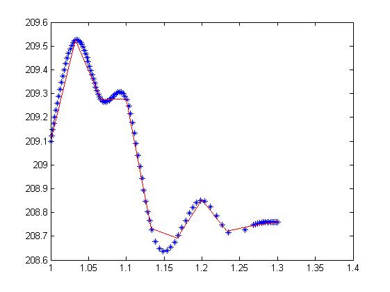
pointInput=[1 209.1;1.033 209.525;1.067 209.273;1.1 209.277;
    1.133 208.734;1.167 208.693;1.2 208.852;1.233 208.722;1.267 208.746;1.3 208.759];

The distribution of these points is shown in the red disconnection in the figure below (not the blue * point, but the blue curve I finally fit).

② calculate the equivalence of N, N and k

N is the number of interpolation points. There are 10 interpolation points on it, so N=10. The number of control points is N+2. n=N+1. K is the degree, here is a cubic B-spline curve, so k=3. MATLAB code:

N=length(pointInput);
k=3;
n=N-1;

③ Inverse control point

Here, we mainly refer to the contents in the PPT in reference [1]. Please check the PPT for details. The expression (1) of cubic B-spline curve is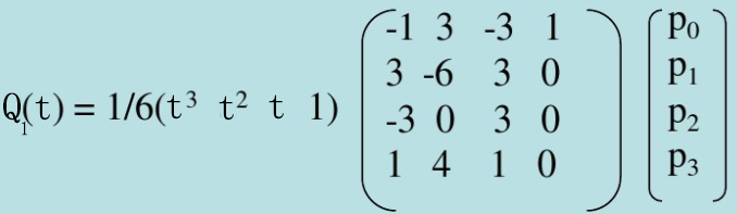

Among themIs the expression of the i-th curve,Is a local parameter,This is the i-th control point. Pay attention to the differences between nodes, node vectors, overall parameters and local parameters (see data [3] or other relevant data for details, which may require a long discussion ~).

For inverse calculation of control points, I use the third boundary condition, as shown in the following figure

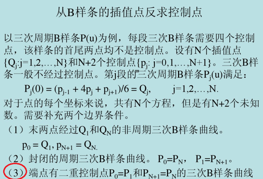
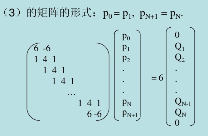
After adding boundary conditions, the matrix equation shown in the figure below can be obtained. In fact, the matrix equation below is obtained from expression (1). For details, please refer to PPT in reference [1] (note that coefficient 6 in the expression should not be omitted).

 

For two-dimensional points, I want to find the B-spline curves in x and y coordinates, so I use two sets of matrix equations to solve their respective control points (for three-dimensional points, I can also find the B-spline curves in z coordinates in the same way). MATLAB code:

%①Ask first x,y Coordinates. If it is a three-dimensional point, it is also required z
b1=[0;pointInput(:,1);0]*6;%Attention coefficient
px=Chase_method(A1,b1);%All control points are obtained by the pursuit method
b2=[0;pointInput(:,2);0]*6;
py=Chase_method(A1,b2);

Chase method is used to find the solution of tridiagonal matrix_ Method (you can directly use commonBut the catch-up method is used here with lower time complexity), and its MATLAB code:

function [ x ] = Chase_method( A, b )
%Chase method Solution of tridiagonal matrix by pursuit method
%   A Is the coefficient of tridiagonal matrix, b Is the constant term at the right end of the equation and returns the value x That is the final solution
%   Note: A As square as possible, b Must be a column vector
%% Find out what is needed by the catch-up method L and U
T = A;
for i = 2 : size(T,1)
    T(i,i-1) = T(i,i-1)/T(i-1,i-1);
    T(i,i) = T(i,i) - T(i-1,i) * T(i,i-1);
end
L = zeros(size(T));
L(logical(eye(size(T)))) = 1;   %Diagonal Assignment 1
for i = 2:size(T,1)
    for j = i-1:size(T,1)
        L(i,j) = T(i,j);
        break;
    end
end
U = zeros(size(T));
U(logical(eye(size(T)))) = T(logical(eye(size(T))));
for i = 1:size(T,1)
    for j = i+1:size(T,1)
        U(i,j) = T(i,j);
        break;
    end
end
%% utilize matlab Ergodic direct solution of matrix equation
y = L\b;
x = U\y;
end

④ Determine node vector

The node vector is the basis for segmenting a segmented B-spline curve (see the following data [3] or other corresponding data). I use the Hadley Judd method to determine the node vector(there are n+k+2 node vectors in total. Note that this is a lowercase n instead of an uppercase n), that is, the first k+1 node in the node vector takes 0, the last k+1 node takes 1, the repeatability is k+1, and then the middle nodeCalculated by Hadley Judd method. Matlab code (note that the subscript of MATLAB array and matrix starts from 1, which is different from 0 in the formula):

%Determine node vector
u=zeros(1,N+1+k+2);%0:1/(N+1+k+2-1):1;
for i=1:k+1
   u(length(u)-i+1)=1;
end
l=zeros(1,N+1);%Control the length of each side of the polygon
for i=1:N+1
    %Note that if three-dimensional points are used, they need to be modified here
   l(i)=sqrt((px(i+1)-px(i))^2+(py(i+1)-py(i))^2);
end
sum1=0;%With Hadley-Judd method determines the node vector
for g=k+1:N+1+1
    for j=g-k:g-1
        sum1=sum1+l(j);
    end
end
for i=k+2:N+2
   u(i)=sum(l(i-k:i-1))/sum1+u(i-1);
end

All control points and node vectors have been calculated, and the expression of the segmented B-spline curve can be known. Next, enter a point to test. In fact, the piecewise B-spline curve is expressed by the parameter equation, and the x and y coordinates are expressed by the parameter U. at the same time, each node in the node vector is taken as the boundary of the piecewise curve segment. The monotonicity of the elements in U does not decrease, and the latter element is not less than one element. The following MATLAB code takes u as the test point uTest, and then finds out which segment uTest belongs to, and calculates that uTest belongs to the score segment:

uTest=0.5;
score=find(uTest>=u,1,'last');%Determine the segment to which the parameter value of the parameter equation belongs
if uTest==1 score=find(u==1,1)-1;end
score=score-k;%Represents the second score Segment spline

Between finding the x and y coordinate values corresponding to the parameter uTest with expression (1), it is necessary to convert the global variable uTest into the local variable t. Note that the value range of uTest in the overall spline curve is [0,1], while the value range of T in the score piecewise curve is [0,1]. The conversion formula is(Is the I + 1st element in the node vector, and meets, where i can be determined by score), the matrix in expression (1) is obtained, MATLAB code:

uNode=1;%above uTest It is a global parameter, which is used to determine which curve it is, and the global parameters should be converted into local parameters t
t=(uTest-u(score+k))/(u(score+1+k)-u(score+k));
for i=1:k
    uNode=[t^i uNode];
end

Calculation of matrix composed of 4x4 matrix and control points in the expression, MATLAB code:

A2=[-1 3 -3 1;
    3 -6 3 0;
    -3 0 3 0;
    1 4 1 0];
QControlx=[];
QControly=[];
for i=1:k+1
    QControlx=[QControlx px(score+i-1)];%The control point is known from the number of segments
    QControly=[QControly py(score+i-1)];
end
QControlx=QControlx.';
QControly=QControly.';

Finally, the desired x and y coordinate values are obtained from the test point uTest. MATLAB code:

Qx=1/6*uNode*A2*QControlx;
Qy=1/6*uNode*A2*QControly;

Attach all MATLAB programs:

%Three times B Spline interpolation, given the interpolation points and two boundary conditions, the control points are inversely calculated, and the piecewise curve is obtained from the control points
%3D point(x,y,z)And 2D points(x,y)The interpolation algorithm is similar to that of, which controls the length of each side of the polygon l To be modified
%pointInput Interpolation point
pointInput=[1 209.1;1.033 209.525;1.067 209.273;1.1 209.277;
    1.133 208.734;1.167 208.693;1.2 208.852;1.233 208.722;1.267 208.746;1.3 208.759];
%pointInput=[0 10;5 8.66;10 0];
%Using the third boundary condition https://wenku.baidu.com/view/2482396e011ca300a6c390b3.html
N=length(pointInput);
k=3;
A1=eye(N+2,N+2)*4;
A1(1,1)=6;A1(1,2)=-6;A1(N+2,N+1)=6;A1(N+2,N+2)=-6;
for i=2:N+1
   A1(i,i-1)=1;A1(i,i+1)=1;
end
%①Ask first x,y Coordinates. If it is a three-dimensional point, it is also required z
b1=[0;pointInput(:,1);0]*6;%Attention coefficient
px=Chase_method(A1,b1);%All control points are obtained by the pursuit method
b2=[0;pointInput(:,2);0]*6;
py=Chase_method(A1,b2);
%Determine node vector
u=zeros(1,N+1+k+2);%0:1/(N+1+k+2-1):1;
for i=1:k+1
   u(length(u)-i+1)=1;
end
l=zeros(1,N+1);%Controls the length of each side of the polygon
for i=1:N+1
    %Note that if three-dimensional points are used, they need to be modified here
   l(i)=sqrt((px(i+1)-px(i))^2+(py(i+1)-py(i))^2);
end
sum1=0;%With Hadley-Judd method determines the node vector
for g=k+1:N+1+1
    for j=g-k:g-1
        sum1=sum1+l(j);
    end
end
for i=k+2:N+2
   u(i)=sum(l(i-k:i-1))/sum1+u(i-1);
end
%Evaluation with basis function
%uTestArray=0:0.01:1;
for uTest=0:0.01:1
%uTest=0.5;
%u3Array=[uTest^3 uTest^2 uTest 1];%Three times B Spline exclusive
score=find(uTest>=u,1,'last');%Determine the segment to which the parameter value of the parameter equation belongs
if uTest==1 score=find(u==1,1)-1;end
score=score-k;%Represents the second score Segment spline
A2=[-1 3 -3 1;
    3 -6 3 0;
    -3 0 3 0;
    1 4 1 0];
QControlx=[];
QControly=[];
for i=1:k+1
    QControlx=[QControlx px(score+i-1)];%The control point is known from the number of segments
    QControly=[QControly py(score+i-1)];
end
uNode=1;%above uTest It is a global parameter, which is used to determine which curve it is, and the global parameters should be converted into local parameters t
t=(uTest-u(score+k))/(u(score+1+k)-u(score+k));
for i=1:k
    uNode=[t^i uNode];
end
QControlx=QControlx.';
QControly=QControly.';
Qx=1/6*uNode*A2*QControlx;
Qy=1/6*uNode*A2*QControly;
plot(Qx,Qy,'*');hold on;
end
plot(pointInput(:,1),pointInput(:,2),'r');

function [ x ] = Chase_method( A, b )
%Chase method Solution of tridiagonal matrix by pursuit method
%   A Is the coefficient of tridiagonal matrix, b Is the constant term at the right end of the equation and returns the value x That is the final solution
%   Note: A As square as possible, b Must be a column vector
%% Find out what is needed by the catch-up method L and U
T = A;
for i = 2 : size(T,1)
    T(i,i-1) = T(i,i-1)/T(i-1,i-1);
    T(i,i) = T(i,i) - T(i-1,i) * T(i,i-1);
end
L = zeros(size(T));
L(logical(eye(size(T)))) = 1;   %Diagonal Assignment 1
for i = 2:size(T,1)
    for j = i-1:size(T,1)
        L(i,j) = T(i,j);
        break;
    end
end
U = zeros(size(T));
U(logical(eye(size(T)))) = T(logical(eye(size(T))));
for i = 1:size(T,1)
    for j = i+1:size(T,1)
        U(i,j) = T(i,j);
        break;
    end
end
%% utilize matlab Ergodic direct solution of matrix equation
y = L\b;
x = U\y;
end

In the effect drawing, the blue points are curve fitting points, and the red disconnection is composed of interpolation points: