5.1 Classification learning

The qualitative output of Classification problem is Classification, or discrete variable prediction.
Regression problem, the quantitative output is regression, or continuous variable prediction.

"""
Please note, this code is only for python 3+. If you are using python 2+, please modify the code accordingly.
"""
from __future__ import print_function #Enforce the syntax of python 3, regardless of the version of python in your environment
import tensorflow as tf
from tensorflow.examples.tutorials.mnist import input_data #Import mnist Library
# number 1 to 10 data
mnist = input_data.read_data_sets('MNIST_data', one_hot=True) #If there is no mnist data, download it; Use one_hot coding

def add_layer(inputs, in_size, out_size, activation_function=None,): #Neural network function
    # add one more layer and return the output of this layer
    Weights = tf.Variable(tf.random_normal([in_size, out_size]))
    biases = tf.Variable(tf.zeros([1, out_size]) + 0.1,)
    Wx_plus_b = tf.matmul(inputs, Weights) + biases
    if activation_function is None:
        outputs = Wx_plus_b
    else:
        outputs = activation_function(Wx_plus_b)
    return outputs

def compute_accuracy(v_xs, v_ys): #Calculation accuracy function
    global prediction #Define global variables in functions
    y_pre = sess.run(prediction, feed_dict={xs: v_xs}) 
    correct_prediction = tf.equal(tf.argmax(y_pre,1), tf.argmax(v_ys,1)) #Function TF Equal (x, y, name = none) compares the equal elements in the matrix / vector of X and y, returns True if they are equal, False if they are not equal, and the dimension of the returned matrix / vector is the same as that of X; tf.argmax() returns the subscript corresponding to the maximum value (1 for each column and 0 for each row)
    accuracy = tf.reduce_mean(tf.cast(correct_prediction, tf.float32)) #tf.cast() type conversion function, which will correct_ Convert prediction to float32 type and correct_prediction find the average value to arrive at arrulacy
    result = sess.run(accuracy, feed_dict={xs: v_xs, ys: v_ys})
    return result

# define placeholder for inputs to network
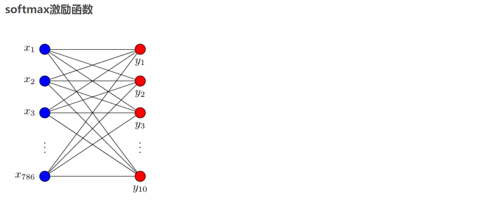
xs = tf.placeholder(tf.float32, [None, 784]) #The input is N pictures, and each picture is composed of 28x28=784 pixels
ys = tf.placeholder(tf.float32, [None, 10]) #Output N data, each picture identifies a number 0-9, a total of 10 kinds

# add output layer
prediction = add_layer(xs, 784, 10,  activation_function=tf.nn.softmax) #Input 784, output 10, excitation function using softmax

# the error between prediction and real data
cross_entropy = tf.reduce_mean(-tf.reduce_sum(ys * tf.log(prediction),
                                              reduction_indices=[1])) #The cross entropy function is selected as the loss function (i.e. the optimization objective function). Cross entropy is used to measure the similarity between the predicted value and the real value. If they are exactly the same, their cross entropy is equal to zero.
train_step = tf.train.GradientDescentOptimizer(0.5).minimize(cross_entropy) #Gradient descent method

sess = tf.Session()
# important step
# tf.initialize_all_variables() no long valid from
# 2017-03-02 if using tensorflow >= 0.12
if int((tf.__version__).split('.')[1]) < 12 and int((tf.__version__).split('.')[0]) < 1:
    init = tf.initialize_all_variables()
else:
    init = tf.global_variables_initializer()
sess.run(init)
#sess.run(tf.global_variables_initializer()) #Initialization model parameters

for i in range(1000): #train
    batch_xs, batch_ys = mnist.train.next_batch(100) #100 pictures are used for training each time to avoid too large annual data and too slow training
    sess.run(train_step, feed_dict={xs: batch_xs, ys: batch_ys})
    if i % 50 == 0:
        print(compute_accuracy(
            mnist.test.images, mnist.test.labels)) #For the test set, images is the input and labels is the output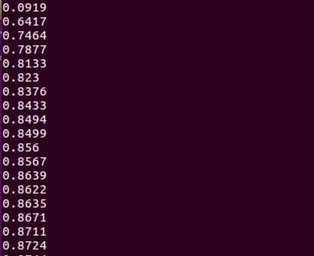

About MNIST Library:

MNIST library is a handwritten numeral library, containing 55000 training pictures, and the resolution of each picture is 28 × 28.

 

from tensorflow.examples.tutorials.mnist import input_data
mnist = input_data.read_data_sets("MNIST_data/", one_hot=True)

print(mnist.train.images.shape) #train
print(mnist.train.labels.shape) 
print(mnist.validation.images.shape) #check
print(mnist.validation.labels.shape)
print(mnist.test.images.shape) #test
print(mnist.test.labels.shape)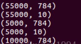

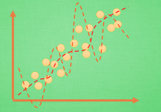
5.2 what is overfitting

Over fitting = conceit (learning is too good, but practical application is not applicable)

For a classification problem, through learning and training neural network Get a straight line / curve to distinguish the origin of the two colors. The error of the learned curve may be large or small.

 

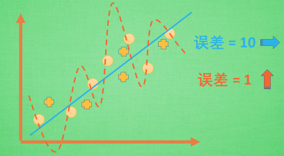
Of course, the small error can only show that the effect will be very good for the given training set, but if in practical application or given another set of test sets, its effect may become very poor.

terms of settlement
There are only two solutions
The first is to increase the data set and give more data to the neural network for learning and training to get a more accurate classification curve. Most of the over fitting problems are due to the insufficient amount of data. If we have thousands of data, the red line will slowly be straightened and become less distorted.

terms of settlement

There are only two solutions
The first is to increase the data set and give more data to the neural network for learning and training to get a more accurate classification curve. Most of the over fitting problems are due to the insufficient amount of data. If we have thousands of data, the red line will slowly be straightened and become less distorted.

The second is to use some methods to prevent over fitting, such as L1, L2 ··········································································.
The key formula for simplifying machine learning is y=Wx, and W is the various parameters that the machine needs to learn. In over fitting, the value of W often changes very large or very small. In order not to make w change too much, we do some tricks on the calculation error. Original cost = predicted value - the square of the real value. If w becomes too large, we will make cost become larger and become a punishment mechanism. So we consider w himself. Here abs is absolute.
Other L2, L3 and L4 are also replaced by square cube and 4th power, etc. With these methods, we can ensure that the learned lines will not be too distorted.

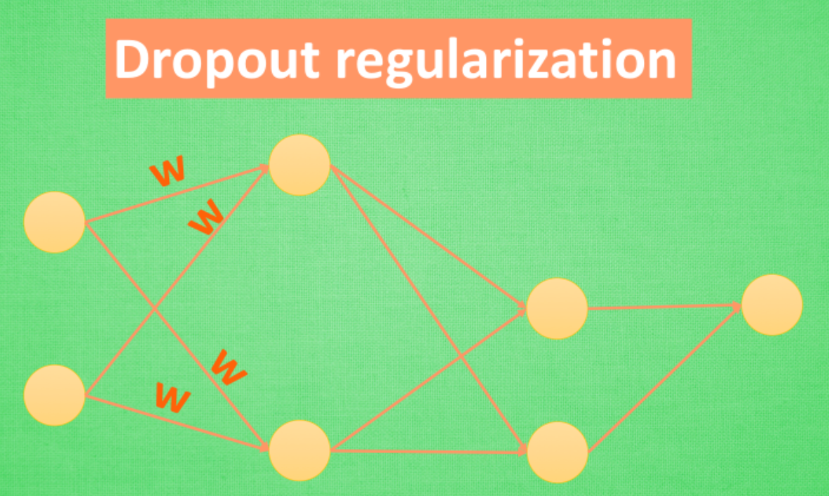
Dropout method is a method specially used for neural network. Before training, some neurons in the hidden layer are randomly deleted to form an incomplete neural network for training. Before the second training, it is restored to a complete neural network, and then some neurons are randomly deleted, Another incomplete training. The purpose of this is that each prediction result will not depend on some specific neurons. Like the normalization of L1 and L2, the over dependent W, that is, the value of training parameters will be large, and L1 and L2 will punish these large parameters. Dropout's approach is to fundamentally prevent neural networks from being overly dependent.

 

5.3 Dropout solution overfitting

from __future__ import print_function
import tensorflow as tf
from sklearn.datasets import load_digits
from sklearn.model_selection import train_test_split
from sklearn.preprocessing import LabelBinarizer

# load data
digits = load_digits()
X = digits.data
y = digits.target
y = LabelBinarizer().fit_transform(y)
X_train, X_test, y_train, y_test = train_test_split(X, y, test_size=.3)


def add_layer(inputs, in_size, out_size, layer_name, activation_function=None, ):
    # add one more layer and return the output of this layer
    Weights = tf.Variable(tf.random_normal([in_size, out_size]))
    biases = tf.Variable(tf.zeros([1, out_size]) + 0.1, )
    Wx_plus_b = tf.matmul(inputs, Weights) + biases
    # here to dropout
    Wx_plus_b = tf.nn.dropout(Wx_plus_b, keep_prob)
    if activation_function is None:
        outputs = Wx_plus_b
    else:
        outputs = activation_function(Wx_plus_b, )
    tf.summary.histogram(layer_name + '/outputs', outputs)
    return outputs


# define placeholder for inputs to network
keep_prob = tf.placeholder(tf.float32)
xs = tf.placeholder(tf.float32, [None, 64])  # 8x8
ys = tf.placeholder(tf.float32, [None, 10])

# add output layer
l1 = add_layer(xs, 64, 50, 'l1', activation_function=tf.nn.tanh)
prediction = add_layer(l1, 50, 10, 'l2', activation_function=tf.nn.softmax)

# the loss between prediction and real data
cross_entropy = tf.reduce_mean(-tf.reduce_sum(ys * tf.log(prediction),
                                              reduction_indices=[1]))  # loss
tf.summary.scalar('loss', cross_entropy)
train_step = tf.train.GradientDescentOptimizer(0.5).minimize(cross_entropy)

sess = tf.Session()
merged = tf.summary.merge_all()
# summary writer goes in here
train_writer = tf.summary.FileWriter("logs/train", sess.graph)
test_writer = tf.summary.FileWriter("logs/test", sess.graph)

# tf.initialize_all_variables() no long valid from
# 2017-03-02 if using tensorflow >= 0.12
if int((tf.__version__).split('.')[1]) < 12 and int((tf.__version__).split('.')[0]) < 1:
    init = tf.initialize_all_variables()
else:
    init = tf.global_variables_initializer()
sess.run(init)
for i in range(500):
    # here to determine the keeping probability
    sess.run(train_step, feed_dict={xs: X_train, ys: y_train, keep_prob: 0.5})
    if i % 50 == 0:
        # record loss
        train_result = sess.run(merged, feed_dict={xs: X_train, ys: y_train, keep_prob: 1})
        test_result = sess.run(merged, feed_dict={xs: X_test, ys: y_test, keep_prob: 1})
        train_writer.add_summary(train_result, i)
        test_writer.add_summary(test_result, i)

5.4 what is convolutional neural network (CNN)
5.5 CNN convolutional neural network 1
5.6 CNN convolutional neural network 2
5.7 CNN convolutional neural network 3
5.8 save read
5.9 what is recurrent neural network (RNN)
5.10 what is LSTM recurrent neural network
5.11 RNN cyclic neural network
5.12 RNN LSTM recurrent neural network (classification example)
5.13 RNN LSTM (regression example)
Rntm 14.5 regression example
5.15 what is autoencoder
5.16 self coding Autoencoder (unsupervised learning)
5.17 scope naming method
5.18 what is batch normalization
5.19 Batch Normalization
5.20 Tensorflow 2017 update
5.21 visualization of gradient descent with Tensorflow
5.22 what is Transfer Learning
5.23 Transfer Learning