1, What is a fully connected neural network?

Fully connected neural network, as the name implies, is a connection between any two nodes between two adjacent layers. Fully connected neural network is the most common model (for example, compared with CNN). Because it is fully connected, it will have more weight values and connections, so it also means more memory and calculation.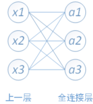

Each node of the full connection layer is connected with all nodes of the previous layer, which is used to integrate the features extracted from the front edge. Because of its fully connected characteristics, the parameters of the general fully connected layer are also the most.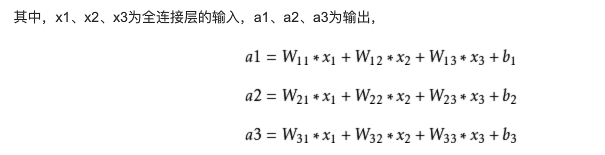

2, What is MNIST?

MNIST is an entry-level computer vision data set, which contains a variety of handwritten digital pictures: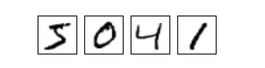

It also contains the label corresponding to each picture, which tells us the number. For example, the labels of the above four pictures are 5, 0, 4, 1.
We will train a machine learning model to predict the number in the picture. So, we will start with a very simple mathematical model, which is called Softmax Regression.

3, MNIST dataset acquisition:

1. To download a dataset:

The official website of MNIST dataset is: Click to open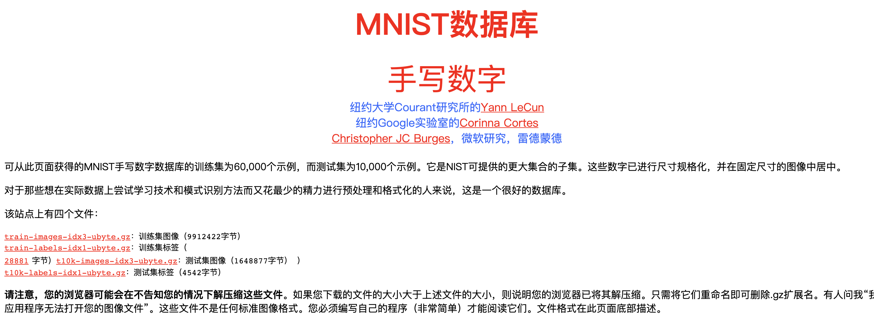

The downloaded dataset is divided into two parts: 60000 rows of training dataset (mnist.train) and 10000 rows of test dataset (mnist.test). Such segmentation is very important. When designing a machine learning model, there must be a separate test data set that is not used for training but for evaluating the performance of the model, so it is easier to extend the designed model to other data sets (generalization).

As mentioned earlier, each MNIST data unit consists of two parts: a picture containing handwritten numbers and a corresponding label. We set these pictures to "xs" and these labels to "ys". Both the training data set and the test data set contain xs and ys. For example, the picture of the training data set is mnist.train.images, and the label of the training data set is mnist.train.labels.

We can also directly run the following code in python environment to generate dataset files
Copy the following code and put it into the python folder and name it: input_data.py

from __future__ import absolute_import
from __future__ import division
from __future__ import print_function
import gzip
import os
import tensorflow.python.platform
import numpy
from six.moves import urllib
from six.moves import xrange  # pylint: disable=redefined-builtin
import tensorflow as tf
SOURCE_URL = 'http://yann.lecun.com/exdb/mnist/'
def maybe_download(filename, work_directory):
  """Download the data from Yann's website, unless it's already here."""
  if not os.path.exists(work_directory):
    os.mkdir(work_directory)
  filepath = os.path.join(work_directory, filename)
  if not os.path.exists(filepath):
    filepath, _ = urllib.request.urlretrieve(SOURCE_URL + filename, filepath)
    statinfo = os.stat(filepath)
    print('Successfully downloaded', filename, statinfo.st_size, 'bytes.')
  return filepath
def _read32(bytestream):
  dt = numpy.dtype(numpy.uint32).newbyteorder('>')
  return numpy.frombuffer(bytestream.read(4), dtype=dt)[0]
def extract_images(filename):
  """Extract the images into a 4D uint8 numpy array [index, y, x, depth]."""
  print('Extracting', filename)
  with gzip.open(filename) as bytestream:
    magic = _read32(bytestream)
    if magic != 2051:
      raise ValueError(
          'Invalid magic number %d in MNIST image file: %s' %
          (magic, filename))
    num_images = _read32(bytestream)
    rows = _read32(bytestream)
    cols = _read32(bytestream)
    buf = bytestream.read(rows * cols * num_images)
    data = numpy.frombuffer(buf, dtype=numpy.uint8)
    data = data.reshape(num_images, rows, cols, 1)
    return data
def dense_to_one_hot(labels_dense, num_classes=10):
  """Convert class labels from scalars to one-hot vectors."""
  num_labels = labels_dense.shape[0]
  index_offset = numpy.arange(num_labels) * num_classes
  labels_one_hot = numpy.zeros((num_labels, num_classes))
  labels_one_hot.flat[index_offset + labels_dense.ravel()] = 1
  return labels_one_hot
def extract_labels(filename, one_hot=False):
  """Extract the labels into a 1D uint8 numpy array [index]."""
  print('Extracting', filename)
  with gzip.open(filename) as bytestream:
    magic = _read32(bytestream)
    if magic != 2049:
      raise ValueError(
          'Invalid magic number %d in MNIST label file: %s' %
          (magic, filename))
    num_items = _read32(bytestream)
    buf = bytestream.read(num_items)
    labels = numpy.frombuffer(buf, dtype=numpy.uint8)
    if one_hot:
      return dense_to_one_hot(labels)
    return labels
class DataSet(object):
  def __init__(self, images, labels, fake_data=False, one_hot=False,
               dtype=tf.float32):
    """Construct a DataSet.
    one_hot arg is used only if fake_data is true.  `dtype` can be either
    `uint8` to leave the input as `[0, 255]`, or `float32` to rescale into
    `[0, 1]`.
    """
    dtype = tf.as_dtype(dtype).base_dtype
    if dtype not in (tf.uint8, tf.float32):
      raise TypeError('Invalid image dtype %r, expected uint8 or float32' %
                      dtype)
    if fake_data:
      self._num_examples = 10000
      self.one_hot = one_hot
    else:
      assert images.shape[0] == labels.shape[0], (
          'images.shape: %s labels.shape: %s' % (images.shape,
                                                 labels.shape))
      self._num_examples = images.shape[0]
      # Convert shape from [num examples, rows, columns, depth]
      # to [num examples, rows*columns] (assuming depth == 1)
      assert images.shape[3] == 1
      images = images.reshape(images.shape[0],
                              images.shape[1] * images.shape[2])
      if dtype == tf.float32:
        # Convert from [0, 255] -> [0.0, 1.0].
        images = images.astype(numpy.float32)
        images = numpy.multiply(images, 1.0 / 255.0)
    self._images = images
    self._labels = labels
    self._epochs_completed = 0
    self._index_in_epoch = 0
  @property
  def images(self):
    return self._images
  @property
  def labels(self):
    return self._labels
  @property
  def num_examples(self):
    return self._num_examples
  @property
  def epochs_completed(self):
    return self._epochs_completed
  def next_batch(self, batch_size, fake_data=False):
    """Return the next `batch_size` examples from this data set."""
    if fake_data:
      fake_image = [1] * 784
      if self.one_hot:
        fake_label = [1] + [0] * 9
      else:
        fake_label = 0
      return [fake_image for _ in xrange(batch_size)], [
          fake_label for _ in xrange(batch_size)]
    start = self._index_in_epoch
    self._index_in_epoch += batch_size
    if self._index_in_epoch > self._num_examples:
      # Finished epoch
      self._epochs_completed += 1
      # Shuffle the data
      perm = numpy.arange(self._num_examples)
      numpy.random.shuffle(perm)
      self._images = self._images[perm]
      self._labels = self._labels[perm]
      # Start next epoch
      start = 0
      self._index_in_epoch = batch_size
      assert batch_size <= self._num_examples
    end = self._index_in_epoch
    return self._images[start:end], self._labels[start:end]
def read_data_sets(train_dir, fake_data=False, one_hot=False, dtype=tf.float32):
  class DataSets(object):
    pass
  data_sets = DataSets()
  if fake_data:
    def fake():
      return DataSet([], [], fake_data=True, one_hot=one_hot, dtype=dtype)
    data_sets.train = fake()
    data_sets.validation = fake()
    data_sets.test = fake()
    return data_sets
  TRAIN_IMAGES = 'train-images-idx3-ubyte.gz'
  TRAIN_LABELS = 'train-labels-idx1-ubyte.gz'
  TEST_IMAGES = 't10k-images-idx3-ubyte.gz'
  TEST_LABELS = 't10k-labels-idx1-ubyte.gz'
  VALIDATION_SIZE = 5000
  local_file = maybe_download(TRAIN_IMAGES, train_dir)
  train_images = extract_images(local_file)
  local_file = maybe_download(TRAIN_LABELS, train_dir)
  train_labels = extract_labels(local_file, one_hot=one_hot)
  local_file = maybe_download(TEST_IMAGES, train_dir)
  test_images = extract_images(local_file)
  local_file = maybe_download(TEST_LABELS, train_dir)
  test_labels = extract_labels(local_file, one_hot=one_hot)
  validation_images = train_images[:VALIDATION_SIZE]
  validation_labels = train_labels[:VALIDATION_SIZE]
  train_images = train_images[VALIDATION_SIZE:]
  train_labels = train_labels[VALIDATION_SIZE:]
  data_sets.train = DataSet(train_images, train_labels, dtype=dtype)
  data_sets.validation = DataSet(validation_images, validation_labels,
                                 dtype=dtype)
  data_sets.test = DataSet(test_images, test_labels, dtype=dtype)
  return data_sets

2. Import database:

Then we can use the import dataset

import input_data
mnist = input_data.read_data_sets("MNIST_data/", one_hot=True)

Each picture contains 28 pixels X28 pixels. We can use an array of numbers to represent this picture: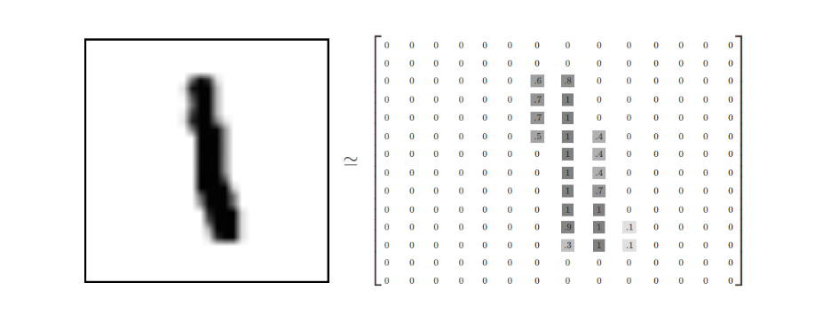

Let's expand this array into a vector with a length of 28x28 = 784. How to expand this array (the order between numbers) is not important, as long as you keep each picture expanded in the same way. From this point of view, the image of MNIST dataset is the point in 784 dimensional vector space, and has a relatively complex structure (Note: the visualization of such data is computationally intensive).

Flattening the digital array of a picture will lose the two-dimensional structure information of the picture. This is obviously not ideal. The best computer vision methods will mine and use these structural information, which we will introduce in the following tutorials. But in this tutorial, we ignore these structures. The simple mathematical model introduced, softmax regression, will not use these structural information.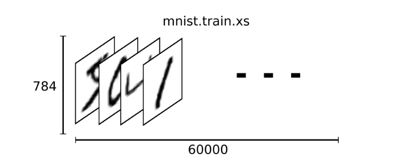

Therefore, in MNIST training data set, mnist.train.images is a tensor with the shape of [60000, 784]. The first dimension number is used to index pictures, and the second dimension number is used to index pixels in each picture. Each element in this tensor represents the intensity value of a pixel in a picture, which is between 0 and 1.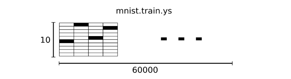

The label of the corresponding MNIST dataset is a number between 0 and 9, which is used to describe the number represented in a given picture. For this tutorial, we make the tag data "one hot vectors.". A one hot vector is zero in all dimensions except one digit. So in this tutorial, the number n will be represented as a 10 dimensional vector with the number 1 only in the nth dimension (starting from 0). For example, tag 0 would be represented as ([1,0,0,0,0,0,0,0,0,0,0]). Therefore, mnist.train.labels is a [60000, 10] number matrix.

4, Building neural networks:

1. We use Softmax regression:

We know that each picture of MNIST represents a number, from 0 to 9. We want to get the probability that a given picture represents each number. For example, our model may speculate that the probability of a picture containing 9 representing the number 9 is 80%, but the probability of judging it as 8 is 5% (because both 8 and 9 have small circles in the upper half), and then give it a smaller value representing other numbers.

This is a classic case of using the softmax regression model. Softmax model can be used to assign probabilities to different objects. Even after that, when we train more refined models, we need to use softmax to allocate the probability in the last step.

softmax regression consists of two steps: the first step

In order to obtain the evidence that a given picture belongs to a specific digital class, we weighted the pixel values of the picture. If the pixel has strong evidence that the image does not belong to this category, the corresponding weight value is negative. On the contrary, if the pixel has favorable evidence to support that the image belongs to this category, the weight value is positive.

The following image shows the weight of each pixel on the image learned by a model for a specific digital class. Red represents the negative weight and blue represents the positive weight.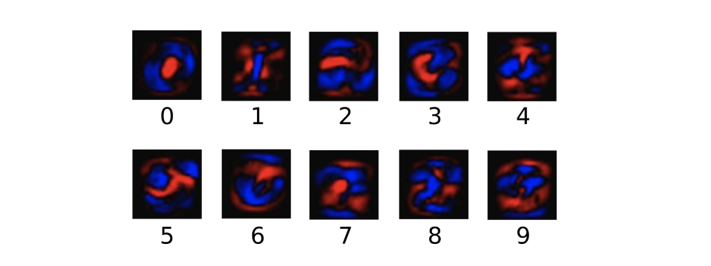

We also need to add an extra bias, because the input often has some irrelevant interference. Therefore, for a given input picture x, the evidence that it represents the number i can be expressed as: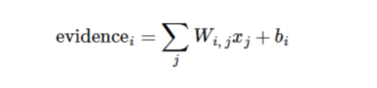

Where, represents the weight, represents the offset of the digital class i, and j represents the pixel index of the given picture x for pixel summation. Then we can use softmax function to convert these evidences into probability y: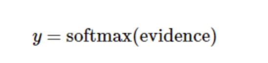

Softmax here can be regarded as an activation function or a link function, which transforms the output of the linear function we defined into the format we want, that is, the probability distribution of 10 digital classes. Therefore, given a picture, its coincidence for each number can be converted into a probability value by softmax function. The softmax function can be defined as: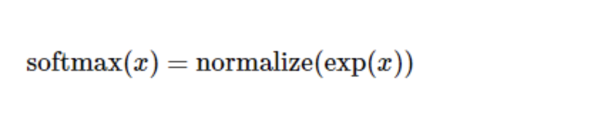

Expand the formula on the right side of the equation to get: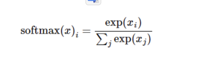

But more often, the softmax model function is defined as the former form: the input value is treated as a power index to evaluate, and then the results are regularized. This power operation indicates that the larger evidence corresponds to the multiplier weight value in the larger hypothesis model. Conversely, having less evidence means having smaller multiplier coefficients in the hypothetical model. Suppose the weight in the model can not be zero or negative. Softmax then regularizes these weight values so that their sum is equal to 1 to construct an effective probability distribution.
For the softmax regression model, the following figure can be used to explain. For the xs weighted sum of the input, add an offset respectively, and finally input it into the softmax function: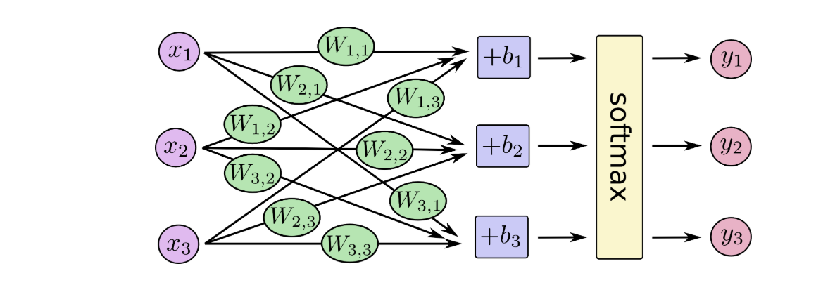

If we write it as an equation, we can get: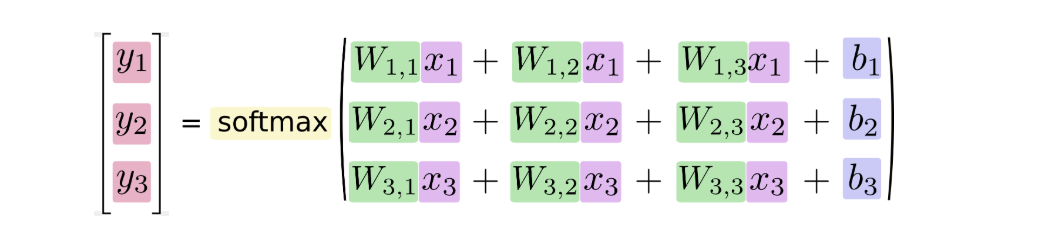

We can also use vectors to represent the calculation process: matrix multiplication and vector addition. This helps to improve the calculation efficiency. (also a more effective way of thinking)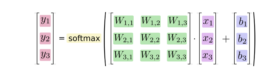

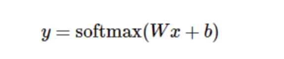
Further, it can be written in a more compact way:

2. Build forward communication:

We describe these interactive operation units by manipulating symbolic variables. We can create one in the following ways:

x = tf.placeholder("float", [None, 784])
y_ = tf.placeholder("float", [None,10])

x and y are not specific values, but placeholder s, which we enter when TensorFlow runs the calculation. We want to be able to input any number of MNIST images, and flatten each image into 784 dimensional vector. We use the 2-dimensional floating-point tensor to represent these graphs. The shape of this tensor is [None, 784]. (None here indicates that the first dimension of this tensor can be of any length.)

Our model also needs weight values and offsets, which we can think of as additional inputs (using placeholders), but TensorFlow has a better way to represent them: Variable. A Variable represents a modifiable tensor, which exists in TensorFlow's diagram for describing interactive operations. They can be used to calculate input values or modified in calculations. For various machine learning applications, there are generally model parameters, which can be represented by variables.

W = tf.Variable(tf.zeros([784,10]))
b = tf.Variable(tf.zeros([10]))

We give tf.Variable different initial values to create different variables: here, we initialize W and b with all zero tensors. Because we need to learn the values of W and b, their initial values can be set at will.

Note that the dimension of W is [784, 10], because we want to multiply the 784 dimensional picture vector by it to get a 10 dimensional evidence value vector, each bit corresponds to a different number class. The shape of b is [10], so we can add it directly to the output.

Now, we can implement our model. Just one line of code!

y = tf.nn.softmax(tf.matmul(x,W) + b)

First of all, we use tf.matmul (x, W) to express x times W, which corresponds to the previous equation, where x is a 2-dimensional tensor with multiple inputs. Then add b and input the sum into the tf.nn.softmax function.

3. Calculate loss function:

After training our model, we first need to define an indicator to evaluate the model is good. In fact, in machine learning, we usually define indicators to show that a model is bad. This indicator is called cost or loss, and then minimize this indicator. But the two approaches are the same.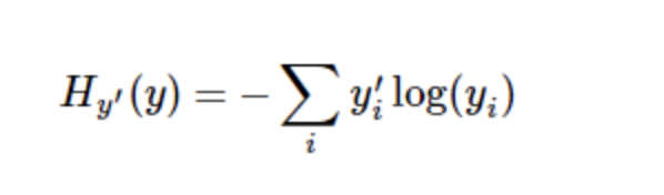

A very common and beautiful cost function is cross entropy. Cross entropy comes from information compression coding technology in information theory, but it has later evolved into an important technical means in other fields from game theory to machine learning.

cross_entropy = -tf.reduce_sum(y_*tf.log(y))

First, tf.log is used to calculate the logarithm of each element of Y. Next, we multiply each element of Y UU by the corresponding element of tf.log(y Uu). Finally, TF. Reduce sum is used to calculate the sum of all elements of the tensor. (note that the cross entropy here is not only used to measure a single pair of predictions and real values, but also the sum of the cross entropy of all 100 pictures. The prediction performance of 100 data points can better describe the performance of our model than that of a single data point.

Now that we know what we need our model to do, it's very easy to train it with TensorFlow. Because TensorFlow has a graph that describes your computing units, it can automatically use the back propagation algorithm to effectively determine how your variables affect the cost value you want to minimize. TensorFlow then uses the optimization algorithm of your choice to constantly modify variables to reduce costs.

train_step = tf.train.GradientDescentOptimizer(0.01).minimize(cross_entropy)

Here, we require TensorFlow to use gradient descent algorithm to minimize cross entropy at a learning rate of 0.01. Gradient descent algorithm is a simple learning process. TensorFlow only needs to move each variable to the direction of reducing cost. Of course, TensorFlow also provides many other optimization algorithms: you can use other algorithms by simply adjusting one line of code.

What TensorFlow actually does here is that it will add a series of new computing operation units to the diagram describing your computing in the background to implement the back propagation algorithm and gradient descent algorithm. Then, what it returns to you is a single operation. When running this operation, it uses gradient descent algorithm to train your model, fine tune your variables, and constantly reduce costs.

Now, we have set up our model. Before running the calculation, we need to add an operation to initialize the variables we created:

init = tf.initialize_all_variables()
with tf.Session() as sess:
	sess.run(init)

Then start training the model. Let's cycle the model 10000 times!
Under Session:

    for i in range(10000):
        batch_xs, batch_ys = mnist.train.next_batch(100)
        sess.run(train_step, feed_dict={x: batch_xs, y_: batch_ys})

In each step of the loop, we randomly grab 100 batch data points from the training data, and then we use these data points as parameters to replace the previous placeholders to run train step.

Using a small amount of random data for training is called stochastic training - in this case, more specifically, random gradient descent training. In an ideal situation, we want to use all our data to train every step, because it can give us better training results, but obviously it needs a lot of computing costs. Therefore, we can use different data subsets for each training, which can not only reduce the computation cost, but also maximize the learning of the overall characteristics of the data set.

4. Evaluate our model:

So what is the performance of our model?

First of all, let's find out the tags that predict correctly. Tf.argmax is a very useful function, which can give the index value of the maximum data value of a sensor object in a certain dimension. Since the label vector is composed of 0,1, the index location of the maximum value 1 is the category label. For example, tf.argmax(y,1) returns the label value predicted by the model for any input x, and tf.argmax(y,1) represents the correct label. We can use tf.equal to detect whether our prediction is true label matching (the index location also represents matching).

correct_prediction = tf.equal(tf.argmax(y,1), tf.argmax(y_,1))

This line of code will give us a set of Boolean values. In order to determine the proportion of correct predictors, we can convert the Boolean value into floating-point number and then take the average value. For example, [True, False, True, True] will change to [1,0,1,1], and take the average value to get 0.75

accuracy = tf.reduce_mean(tf.cast(correct_prediction, "float"))

Finally, we calculate the accuracy of the learned model on the test data set.

print(sess.run(accuracy, feed_dict={x: mnist.test.images, y_: mnist.test.labels}))

The final result should be about 91%.

How's the result? Well, not so good. In fact, the result is very poor. This is because we only use a very simple model. However, with a little improvement, we can get 97% accuracy. The best model can even get more than 99.7% accuracy!

The article draws on the official explanation of Tensorflow