Feature category
Common feature types include: numerical feature, category feature, sequence feature, k-v feature, embedding feature, cross feature, etc.
1. Numerical characteristics
Numerical features are the most common, such as some statistical features: ctr, click_num, etc. in different business scenarios, the amount of numerical features is different. Numerical features can be divided into two categories from the way of obtaining features:
- One is the basic statistical characteristics
- One is to calculate the composite features of output according to certain rules according to business scenarios
Usually, composite features contain more information and are more effective. The common processing methods of numerical characteristics are summarized below.
1.1 characteristic barrel separation
For continuous statistical features such as hits, likes and collections, direct coding will cause a great waste of coding space. Therefore, divide buckets first, and the features in the same bucket share a coding index, which can not only reduce the coding space, but also realize the efficient processing of features. In this way, the continuous features are mapped into N buckets and one hot coding is carried out directly, which is simple and convenient.
Bucket division rule: that is, the determination of bucket division threshold. If the bucket division threshold is set unreasonably, some features will be concentrated in several buckets, which will greatly reduce the discrimination of features
- Equally spaced barrels. However, two points need to be paid attention to in this way:
- Whether the numerical distribution of this feature is average, if the long tail is serious, it is obviously unreasonable;
- Whether the feature outliers have a great impact on barrel division. For example, the maximum value of a fault in the hits will directly squeeze other features into the front barrel, while the back barrel is very sparse.
- Equal frequency bucket Division: first make statistics on the equal points of the data, and then roughly determine the bucket division threshold according to the situation of each characteristic equal point. In this way, the following two principles can be basically guaranteed:
- The characteristic magnitude in each bucket is similar
- The features in each barrel have a certain degree of discrimination
1.2 feature truncation
Outliers may appear in features, which may directly affect the results after feature processing. In this case, using feature truncation and removing outliers can improve the accuracy of features. Truncation involves outlier detection.
1.3 data smoothing
For ratio features, the feature value calculated by the small denominator is more unstable and has low confidence. At this time, it is necessary to smooth the data to make it closer to the real value.
- wilson smoothing
For example, for ctr features, there are three case s:- case1: exposure 100, click 3
- case2: exposure 10000, click 300
- case3: exposure 100000, click 3000
Obviously, the ctr calculated by case3 will be closer to the real value because the exposure base is large enough; The value calculated by case1 is the most unstable. With one more click, the ctr becomes 4%. Therefore, it is necessary to smooth case1 and case2.
This value can be corrected by using wilson smoothing, and its calculation formula is as follows:
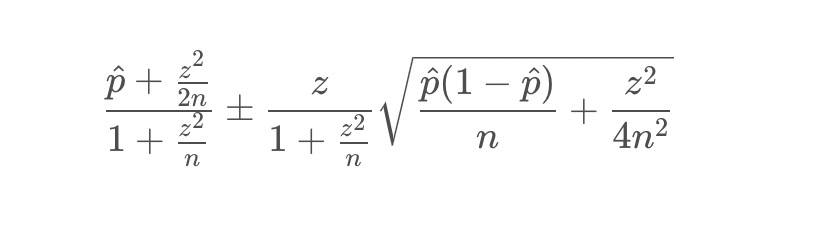
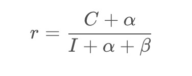
- Bayesian smoothing
1.4 data standardization
- Maximum and minimum standardization
- z-score standardization
2. Basic knowledge of barrel separation
2.1 p quantile
The statistical quadrant is a function
In principle, p can take any value between 0 and 1, but there is a quartile that is more famous in p quantile. The so-called quartile; That is, the values are arranged from small to large and divided into quartiles. The values at the three dividing points are quartiles. Namely: p=0.25, 0.5, 0.75
Method for determining the position of p quantile:
Method 1: pos = (n+1) * p
Method 2: pos = 1+ (n-1)*p
Implementation: through the quantile function in pandas
Function form:
DataFrame.quantile(q=0.5, axis=0, numeric_only=True, interpolation='linear')
Parameters:
- q: float or array-like,the quantile(s) to compute
- axis:0,1, 'index' and 'columns', where 0,' index 'is row wise statistics and 1,' columns' is column wise
- numeric_only: if False, the quantile of datetime and timedelta data will also be calculated.
- Interpolation:
- Linear linear interpolation: i+(j-i)* fraction,fraction is the fractional part of the calculated pos
- lower: i
- higher: j
- nearest: i or j whichever is nearest
- midpoint : (i+j)/2
df = pd.DataFrame(np.array([[1, 1], [2, 10], [3, 100], [4, 100]]),
                  columns=['a', 'b'])
print(df.quantile(0.1))
# Columns of self and the values are the quantities
a    1.3
b    3.7
# Calculation logic: pos = 1 + (4 - 1)*0.1 = 1.3, fraction = 0.3, ret = 1 + (2 - 1) * 0.3 = 1.3
print(df.quantile([0.2, 0.5]))
# Return value: index is Q, the columns are the columns of self, and the values are the quantities
       a     b
0.2  1.6   6.4
0.5  2.5  55.0
2.2 equal width / equal frequency bucket division strategy:
Equal frequency bucket, also known as bucket by quantile, can be realized through pandas Library in order to calculate quantile and map data to quantile box.
- pd.qcut(): select the uniform interval of boxes according to the frequency of these values, that is, the number of numbers contained in each box is the same
pd.qcut(x, q, labels=None, retbins=False, precision=3, duplicates='raise')
- q : int or list-like of float
Number of quantiles. 10 for deciles, 4 for quartiles, etc. Alternately array of quantiles, e.g. [0, .25, .5, .75, 1.] for quartiles.
# Pass in q parameter
factors = np.random.randn(9)
res = pd.qcut(factors, 3)  # Returns the group corresponding to each number
cnt = pd.qcut(factors, 3).value_counts()  # Calculate the number of contained in each group

# Pass in the label parameter
print(pd.qcut(factors, 3, labels=["a", "b", "c"]))  # Returns the group corresponding to each number, but the group name is indicated by label)
print(pd.qcut(factors, 3, labels=False))  # Returns the group corresponding to each number, but displays only the group subscript

# Pass in retbins parameter
print(pd.qcut(factors, 3, retbins=True))  # Return the group corresponding to each number, and additionally return bins, that is, each boundary value
| parameter | explain |
|---|---|
| x | ndarray or Series |
| q | integer, indicating a partitioned array |
| labels | Array or bool, the default is None. When the array is passed in, the name of the group is indicated by label; When False is passed in, only group subscripts are displayed |
| retbins | bool, whether to return bins. The default is False. When True is passed in, additional bins is returned, that is, each boundary value |
| precision | int, precision, default = 3 |
Divide barrels by equal width. Select the uniform spacing of boxes according to the value itself, that is, the spacing of each box is the same
# Pass in the bins parameter
factors = np.random.randn(9)
print(pd.cut(factors, 3))  # Returns the group corresponding to each number
print(pd.cut(factors, bins=[-3, -2, -1, 0, 1, 2, 3]))
print(pd.cut(factors, 3).value_counts())  # Calculate the number of contained in each group

# Pass in label parameter
print(pd.cut(factors, 3, labels=["a", "b", "c"]))  # Returns the group corresponding to each number, but the group name is indicated by label
print(pd.cut(factors, 3, labels=False))  # Returns the group corresponding to each number, but displays only the group subscript
| parameter | explain |
|---|---|
| x | array, only one-dimensional arrays can be used |
| q | integer or sequence of scalars, indicating the divided array or the specified group spacing |
| labels | Array or bool, the default is None. When the array is passed in, the name of the group is indicated by label; When False is passed in, only group subscripts are displayed |
| retbins | bool, whether to return bins. The default is False. When True is passed in, additional bins is returned, that is, each boundary value |
| precision | int, precision, default = 3 |
python_ Equal frequency division box_ Equidistant box
data_temp = data
# Sub box: equidistant equifrequency sub box
# Equidistant box
#bins=10 boxes
data_temp['deposit_cur_balance_bins'] = binning(df = data_temp,col = 'deposit_cur_balance',method='frequency',bins=10)
data_temp['deposit_year_total_balance_bins'] = binning(df = data_temp,col = 'deposit_year_total_balance',method='frequency',bins=10)


def binning(df,col,method,bins):
#     Need to judge the type
    uniqs=df[col].nunique()
    if uniqs<=bins:
        raise KeyError('nunique is smaller than bins: '+col)
#         print('nunique is smaller than bins: '+col)
        return
#     Left open right close
    def ff(x,fre_list):
        if x<=fre_list[0]:
            return 0
        elif x>fre_list[-1]:
            return len(fre_list)-1
        else :
            for i in range(len(fre_list)-1):
                if x>fre_list[i] and x<=fre_list[i+1]:
                    return i
# Equidistant box
    if method=='distance':
        umax=np.percentile(df[col],99.99)
        umin=np.percentile(df[col],0.01)
        step=(umax-umin)/bins
        fre_list=[umin+i*step for i in range(bins+1)]
        return df[col].map(lambda x:ff(x,fre_list))
        #Equal frequency division box
    elif method=='frequency' :
        fre_list=[np.percentile(df[col],100/bins*i) for i in range(bins+1)]
        fre_list=sorted(list(set(fre_list)))
        return df[col].map(lambda x:ff(x,fre_list))
SQL_ Equal frequency division box_ Equidistant box
Equidistant box division / equiwidth box Division: divide the value range of variables into k equal width intervals, and each interval is regarded as a box division.
-- Mathematical operation:yes col Proceed to 0.1(It is divided into 10 points according to equal distance)Width of sub box,Method, first normalize the data to 0-1 Then, the features are divided into corresponding buckets according to the amount of data divided into buckets

---- Equidistant barrel separation  [0.100000,0.590000,1.080000,1.570000,2.060000,2.550000,3.040000,3.530000,4.020000,4.510000,5.000000]

select
    col,
    (col-mi)/(ma-mi) as rate
from
(
    select
        col,
        (select max(col) from  VALUES (5),(4.5), (0.1), (0.15),(0.20), (0.25),(0.3) AS tab(col)) as  ma,
        (select min(col) from  VALUES (5),(4.5), (0.1), (0.15),(0.20), (0.25),(0.3) AS tab(col)) as mi
    from  VALUES (5),(4.5), (0.1), (0.15),(0.20), (0.25),(0.3) AS tab(col)
)
Equal frequency sub box: the observed values are arranged in the order from small to large. According to the number of observations, they are equally divided into k parts. Each part is regarded as a sub box, that is, the concept of percentile.
-- Ntile(n) over(order by col): Block function
-- remarks: NULL Value processing, whether it needs to be a separate group.

select
    col,
    ntile(3) over( order by col) as group1,      -- NULL The default is the minimum value
    if(col is null, null, ntile(3) over( partition by if(col is null, 1, 0) order by col)) as group2     -- take NULL Separate for 1 group
from   VALUES (5), (0.1), (0.15),(0.20), (0.25),(0.3),(null) AS tab(col);
The ntile() function is used to divide the observed values into equal frequency boxes and arrange them in order (ascending order by default). According to the total number of observed values, it is equally divided into k parts. Each part is regarded as a sub box, that is, the concept of percentile. The first or last n% of the data can be selected according to the box number.
Function method: ntile(n) over(order by col) as bucket_numn is the specified number of boxes. If it cannot be evenly distributed, the boxes with smaller numbers will be allocated first, and the number of rows that can be placed in each box can differ by 1 at most. Note: the processing of NULL value can be set as a separate group, or the default value is the minimum value
Supplement:
percent_rank() over(order by col): first get the percentile corresponding to each value, and then divide the boxes according to the actual demand
select  col
        -- Divided by percentile
        , if(group1<0.5, 1, if(group1<=1.0, 2, null)) as group1
        , if(group2<0.5, 1, if(group2<=1.0, 2, null)) as group2
from(
    select  col
            -- NULL The default is the minimum value
            , percent_rank() over( order by col) as group1
            -- take NULL Separate for 1 group
            , if(col is null, null, percent_rank() over( partition by if(col is null, 1, 0) order by col) as group2
    from(
        select cast(col as int) as col
        from(
            select stack(5, 'NULL', '1', '2', '3', '4') as col
        ) as a
    ) as a
) as a