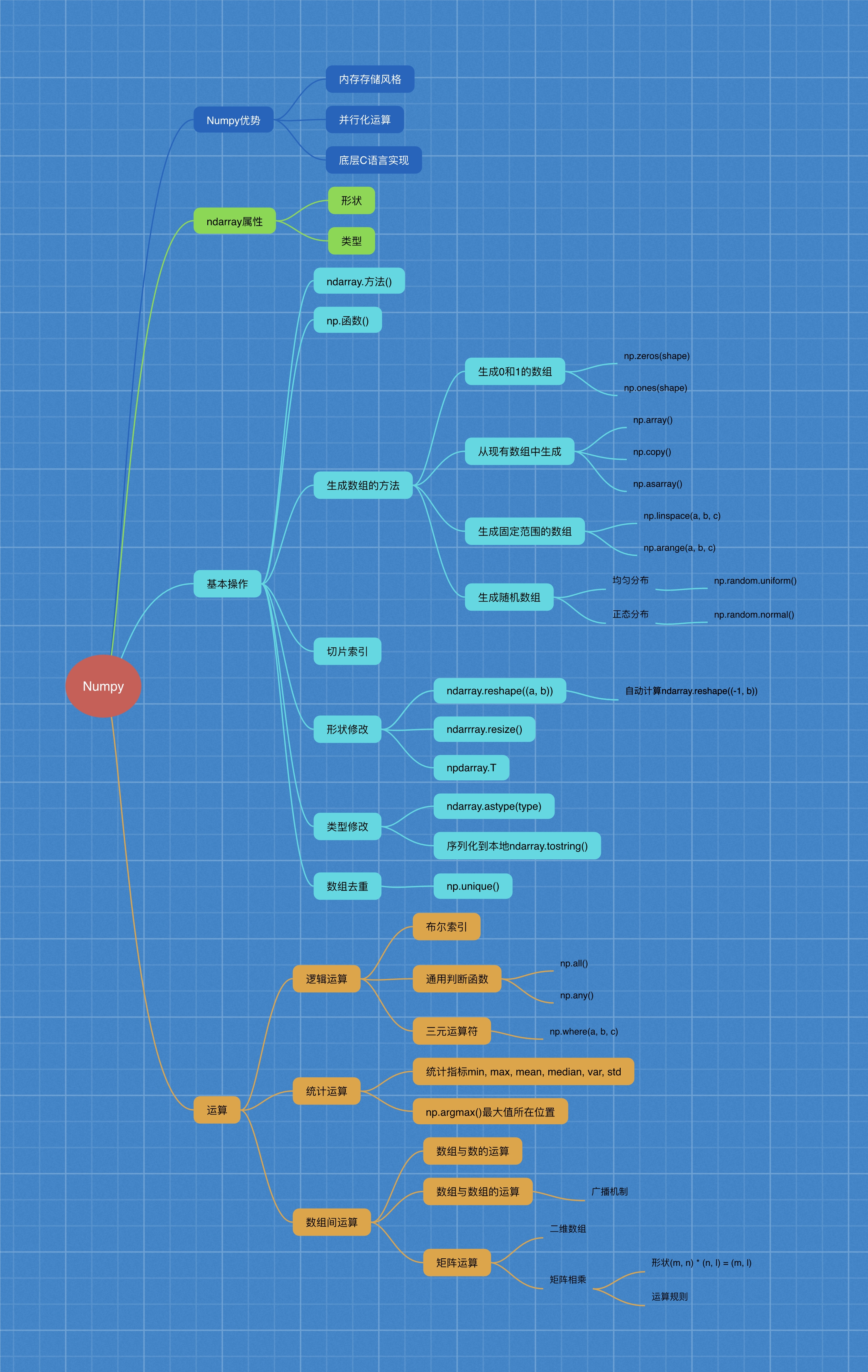
1 Numpy advantage

1.1 introduction to numpy

• Numpy (Numerical Python) is an open-source Python science computing library, which is used to quickly process arrays of any dimension. (numerical → \ to → numerical)
• Numpy supports common array and matrix operations. For the same numerical calculation task, using numpy is much simpler than using Python directly.
• Numpy uses the ndarray object to handle multidimensional arrays, which is a fast and flexible big data container.

1.2 introduction to ndarray

NumPy provides an N-dimensional array type, the ndarray, which describes a collection of "item" of the same type.

NumPy provides an N-dimensional array type, ndarray, which describes a collection of "items" of the same type.

N d array: n → \ to → any; D → \ to → dimension dimension; array → \ to → array

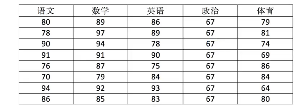
import numpy as np

score = np.array([[80, 89, 86, 67, 79],
[78, 97, 89, 67, 81],
[90, 94, 78, 67, 74],
[91, 91, 90, 67, 69],
[76, 87, 75, 67, 86],
[70, 79, 84, 67, 84],
[94, 92, 93, 67, 64],
[86, 85, 83, 67, 80]])	# Store data in the ndarray container

In[1] : score
Out[1]: array([[80, 89, 86, 67, 79],
           [78, 97, 89, 67, 81],
           [90, 94, 78, 67, 74],
           [91, 91, 90, 67, 69],
           [76, 87, 75, 67, 86],
           [70, 79, 84, 67, 84],
           [94, 92, 93, 67, 64],
           [86, 85, 83, 67, 80]])

In[1] : type(score)
Out[1]: numpy.ndarray   

1.3 comparison of operation efficiency between ndarray and Python native list

Python lists can be used to store one-dimensional arrays, and multi-dimensional arrays can be realized by nesting lists.

So why do you need to use Numpy's ndarray?

import random
import time

# Generate a large array
python_list = []
for i in range(100000000):
    python_list.append(random.random())
ndarray_list = np.array(python_list)

# Sum of native Python list
t1 = time.time()
a = sum(python_list)
t2 = time.time()
d1 = t2 - t1		# 0.7309620380401611

# Darray sum
t3 = time.time()
b = np.sum(ndarray_list)
t4 = time.time()
d2 = t4 - t3		# 0.12980318069458008

1.4 advantages of darray

1. Memory block style: ndarray - the same type - is not universal; list - different types - is universal.
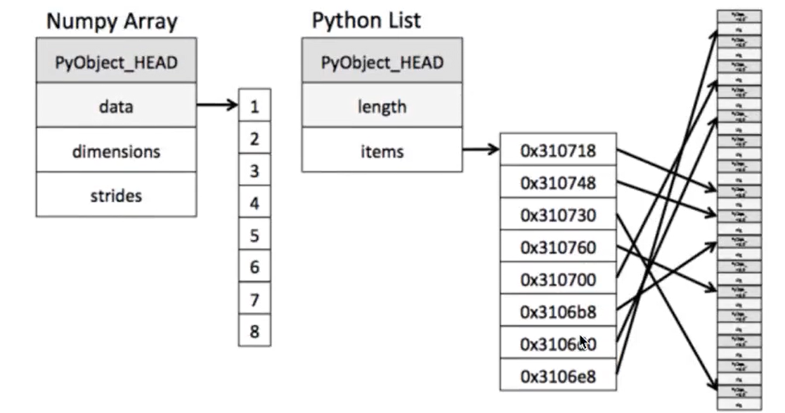
   It can be seen from the figure that when darray stores data, the data and data address are continuous, which makes the batch operation of array elements faster.
    
   Because the types of all elements in ndarray are the same, and the element types in Python list are arbitrary, the memory of ndarray can be continuous when storing elements, while the python native list can only find the next element through addressing, which results in that the ndarray of Numpy is less than that of Python native list in general performance, but in scientific calculation, the ndarray of Numpy is just It can save a lot of loop statements, and the code usage is much simpler than Python native list.

2. Darray supports parallelization (vectorization).

3. The bottom layer of Numpy is written in c language, and GIL (global interpreter lock) is released internally. Its operation speed to array is not limited by Python interpreter, and its efficiency is far higher than pure Python code.

2 N-dimensional array - ndarray

2.1 properties of ndarray

Property name	Attribute interpretation
ndarray.shape	Tuple of array dimension
ndarray.ndim	Array dimension
ndarray.size	Number of elements in array
ndarray.dtype	Type of array element
ndarray.itemsize	Length of an array element (bytes)

In[1] : score.shape
Out[1]: (8, 5)		# 8 rows and 5 columns, tuple representation

In[1] : score.ndim
Out[1]: 2		# 2D

In[1] : score.size
Out[1]: 40		# 40 elements

In[1] : score.dtype
Out[1]: dtype('int64')	# Default integer type

In[1] : score.itemsize
Out[1]: 8		# 8 bytes for one element

2.2 shape of ndarray

# First create some arrays:
a = np.array([[1,2,3],[4,5,6]])
b = np.array([1,2,3,4])
c = np.array([[[1,2,3],[4,5,6]],[[1,2,3],[4,5,6]]])

In[1] : a
Out[1]: array([[1, 2, 3],
           [4, 5, 6]])

In[1] : a.shape
Out[1]: (2, 3)		# Two dimensional array

In[1] : b
Out[1]: array([1, 2, 3, 4])

In[1] : b.shape
Out[1]: (4,)		# One dimensional array

In[1]: c
Out[1]: array([[[1, 2, 3],
            [4, 5, 6]],
    
           [[1, 2, 3],
            [4, 5, 6]]])

In[1] : c.shape
Out[1]: (2, 2, 3)	# 3D array

2.3 types of ndarray

Dtype is numpy.dtype type

name	describe	Shorthand
np.bool	Boolean type stored in one byte (True or False)	'b'
np.int8	One byte size, - 128 to 127	'i'
np.int16	Integer, - 32768 to 32767	'i2'
np.int32	Integer, - 231 to 232-1	'i4'
np.int64	Integer, - 263 to 263-1	'i8'
np.uint8	Unsigned integer, 0 to 255	'u'
np.uint16	Unsigned integer, 0 to 65535	'u2'
np.uint32	Unsigned integer, 0 to 232-1	'u4'
np.uint64	Unsigned integer, 0 to 264-1	'u8'
np.float16	Semi precision floating point number: 16 bits, sign 1 bit, index 5 bits, precision 10 bits	'f2'
np.float32	Single precision floating point number: 32 bits, sign 1 bit, index 8 bits, precision 23 bits	'f4'
np.float64	Double precision floating-point number: 64 bits, sign 1 bit, index 11 bits, precision 52 bits	'f8'
np.complex64	Complex number, two 32-bit floating-point numbers for real part and virtual part respectively	'c8'
np.complex 128	Complex number, two 64 bit floating-point numbers for real part and virtual part respectively	'c16'
np.object	python object	'O'
np.string	character string	'S'
np. unicode_	unicode type	'U'

data = np.array([1.1, 2.2, 3.3])

In[1] : data
Out[1]: array([1.1, 2.2, 3.3])

In[1] : data.dtype
Out[1]: dtype('float64')	# Default floating point type

When creating an array, specify the type:

In[1] : np.array([1.1, 2.2, 3.3], dtype="float32")
Out[1]: array([1.1, 2.2, 3.3], dtype=float32)

In[1] : np.array([1.1, 2.2, 3.3], dtype=np.float32)
Out[1]: array([1.1, 2.2, 3.3], dtype=float32)

# Rarely used
arr = np.array(['python','tensorflow','scikit-learn', 'numpy'], dtype =np.string_)

In[1] : arr
Out[1]: array([b'python', b'tensorflow', b'scikit-learn', b'numpy'], dtype='|S12')

3 basic operation

ndarray. Method () or np. Function name ().

3.1 method of generating array

3.1.1 generate arrays of 0 and 1

• empty(shape[, dtype, order])
  empty_like(a[, dtype, order, subok])
  eye(N[, M, k, dtype, order])
• identity(n[, dtype)
• ones(shape[, dtype, order])
• ones_like(a[, dtype, order, subok])
• zeros(shape[, dtype, order])
  zeros_like(a[, dtype, order, subok])
  full(shape, fill_value[, dtype, order])
• full_like(a, fill_value, dtype, order, subok])

# Generate an array of 0
In[1] : np.zeros(shape=(3, 4), dtype="float32")
Out[1]: array([[0., 0., 0., 0.],
           [0., 0., 0., 0.],
           [0., 0., 0., 0.]], dtype=float32)
# Generate an array of 1
In[1] : np.ones(shape=[2, 3], dtype=np.int32)
Out[1]: array([[1, 1, 1],
           [1, 1, 1]], dtype=int32)

3.1.2 generating from an existing array

• array(object[, dtype, copy, order, subok, ndmin])
• asarray(a[, dtype, order])
• asanyarray(a[, dtype, order])
  ascontiguousarray(a[, dtype])
• asmatrix(data[, dtype)
• copy[a[, order]

On the difference between array and asarray

a = np.array([[1, 2, 3], [4, 5, 6]])

In[1] : a
Out[1]: array([[1, 2, 3],
       [4, 5, 6]])

• np.array(), created from an existing array

a1 = np.array(a)

In[1] : a1
Out[1]: array([[1, 2, 3],
       [4, 5, 6]])

• np.asarray(), equivalent to the form of index, does not really create a new

a2 = np.asarray(a)

In[1] : a2
Out[1]: array([[1, 2, 3],
       [4, 5, 6]])

• np.copy()

a3 = np.copy(a)

In[1] : a3
Out[1]: array([[1, 2, 3],
       [4, 5, 6]])

Modified value:

a[1, 1] = 1000

In[1] : a
Out[1]: array([[   1,    2,    3],
       [   4, 1000,    6]])

• a1 = np.array(a) , data unchanged, deep copy

In[1] : a1
Out[1]: array([[1, 2, 3],
       [4, 5, 6]])

• a2 = np.asarray(a) , data change, shallow copy

In[1] : a2
Out[1]: array([[   1,    2,    3],
       [   4, 1000,    6]])

• a3 = np.copy(score), data unchanged, deep copy

In[1] : data3
Out[1]: array([[1, 2, 3],
       [4, 5, 6]])

3.1.3 generate fixed range array

np.linspace(start, stop, num, endpoint, retstep, dtype)

Generating equispaced sequences

• Start value of start sequence
• stop sequence termination value
  • If endpoint is true, the value is included in the sequence, and the default closed range is []
• num number of evenly spaced samples to generate, default is 50
• Whether the endpoint sequence contains the stop value? The default value is ture
• retstep if true, returns the step size between the sample and consecutive numbers
• dtype output data type of darray

In[1] : np.linspace(0, 10, 5)
Out[1]: array([ 0. ,  2.5,  5. ,  7.5, 10. ])

numpy.arange(start, stop, step, dtype), left close, right open [), step is the step

In[1] : np.arange(0, 10, 5)
Out[1]: array([ 0,  5])

numpy.logspace(start, stop, num, endpoint, base, dtype) to build an equal ratio sequence

3.1.4 generate random array: np.random modular

1. Uniform distribution

One of the important distributions in probability statistics. As the name implies, uniformity means equal possibility. Even distribution is very rare in the natural situation, and the plant community with a certain plant row spacing is even distribution.

• np.random.rand(d0, d1, … dn), returns a set of evenly distributed numbers in [0.0, 1.0]
• np.random.uniform(low=0.0, high=1.0, size=None)
  • Function: random sampling from a uniform distribution [low, high], note that the definition field is left closed and right open
  • Parameter introduction:
    low: lower limit of sampling, float type, default value is 0;
    high: sampling upper bound, float type, default value is 1;
    Size: number of output samples, int or tuple type, for example, size=(m,n,k), output mnk samples, and output 1 value by default.
    Return value: ndarray type, whose shape is consistent with the description in parameter size.
• np.random.randint(low, high=None, size=None, dtype='l')
  • Random sampling from a uniform distribution generates an array of integers or N-dimensional integers. Range: if high is not None, take the random integer between [low, high], otherwise take the random integer between [0, low].

Example:

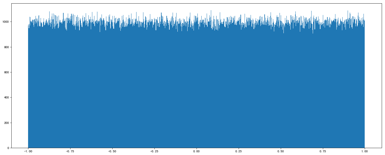
data1 = np.random.uniform(low=-1, high=1, size=1000000)

In[1] : data1
Out[1]: array([-0.49795073, -0.28524454,  0.56473937, ...,  0.6141957 ,
            0.4149972 ,  0.89473129])

Draw a picture to see the distribution:

import matplotlib.pyplot as plt

# 1. Create canvas
plt.figure(figsize=(20, 8), dpi=80)
# 2. Draw histogram
plt.hist(data1, 1000)
# 3. Display image
plt.show()

2. Normal distribution

Introduction:

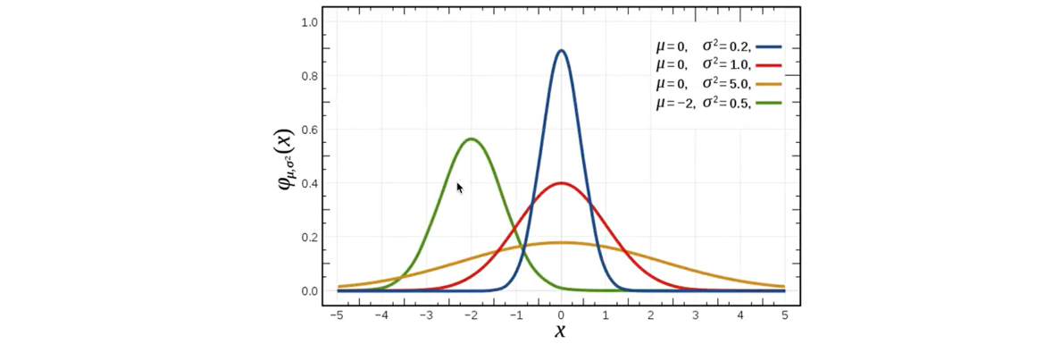
1. Normal distribution is a kind of probability distribution, which is the distribution of continuous random variables with two parameters μ mu μ and σ Sigma σ. The first parameter μ mu μ is the mean value of random variables subject to normal distribution, and the second parameter σ Sigma σ is the standard deviation of this random variable, so the normal distribution is recorded as N(μ, σ) N(\ mu, sigma) N(μ, σ).
   
   Application: the probability distribution of many random Li quantities in life, production and scientific experiments can be approximately described by normal distribution.

2. Characteristics of normal distribution: μ \ mu μ determines the location, and standard deviation σ \ Sigma σ determines the magnitude and concentration of the distribution. When μ = 0\mu=0 μ = 0, σ = 1\sigma=1 σ = 1, the normal distribution is the standard normal distribution.

f(x)=1σ2πe−(x−μ)22σ2f(x) = \frac{1}{\sigma\sqrt{2\pi}}e^{-\frac{(x-\mu)^2}{2\sigma^2}}f(x)=σ2π​1​e−2σ2(x−μ)2​

1. Standard deviation: square root of variance.
   Variance:
   s2=(x1−μ)2+(x2−μ)2+(x3−μ)2+…… +(xn−μ)2ns^2=\frac{(x_1-\mu)^2+(x_2-\mu)^2+(x_3-\mu)^2+…… +(x_n-\mu)^2}{n}s2=n(x1​−μ)2+(x2​−μ)2+(x3​−μ)2+…… +(xn − μ) 2 where μ \ mu μ is the average value, nnn is the total number of data, and sss is the standard deviation σ \ sigma σ
   σ=1N∑i=1N(xi−μ)2\sigma=\sqrt{\frac{1}{N}\sum_{i=1}^N(x_i-\mu)^2} σ = N1 I = 1 Σ n (Xi − μ) 2 significance of standard deviation and variance: a measure of the degree of dispersion of a set of data in probability theory and statistics.

Normal distribution syntax:

• np.random.rand(d0, d1, ... dn)
  • Function: return one or more sample values from the standard normal distribution
• np.random.normal(loc=0.0, scale=1.0, size=None)
  • loc: float type, the mean value of this probability distribution (corresponding to the center of the entire distribution)
  • Scale: float type, the standard deviation of this probability distribution (corresponding to the width of the distribution, the larger the scale is, the fatter it is, the smaller the scale is, the thinner it is)
  • size: int or tuple of ints, the output shape, which is None by default, only outputs one value
• np.random.standard_normal(size=None), returns an array of standard normal distributions of the specified shape.

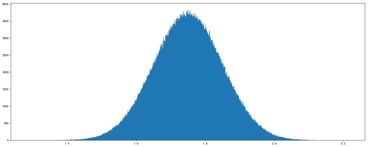
Example:

# Normal distribution
data2 = np.random.normal(loc=1.75, scale=0.1, size=1000000)

In[1] : data2
Out[1]: array([1.66381498, 1.81276401, 1.58393696, ..., 1.72017482, 1.90260969,
           1.69554529])

Image display effect:

# 1. Create canvas
plt.figure(figsize=(20, 8), dpi=80)

# 2. Draw histogram
plt.hist(data2, 1000)

# 3. Display image
plt.show()

3.2 array operation

Case: randomly generate 2-week trading day up and down data of 8 stocks

• Two week trading days: 2 × 5 = 10 days
• Randomly generated up and down in a normal distribution, such as mean 0, variance 1

3.2.1 creation of stock up and down data

stock_change = np.random.normal(loc=0, scale=1, size=(8, 10))

In[1] : stock_change
Out[1]: array([[-0.03469926,  1.68760014,  0.05915316,  2.4473136 , -0.61776756,
            -0.56253866, -1.24738637,  0.48320978,  1.01227938, -1.44509723],
           [-1.8391253 , -1.10142576,  0.09582268,  1.01589092, -1.20262068,
             0.76134643, -0.76782097, -1.11192773,  0.81609586,  0.07659056],
	   ...
           [-2.93762047,  0.22199761,  0.98788788,  0.37899235,  0.28281886,
            -1.75837237, -0.09262863, -0.92354076,  1.11467277,  0.76034531],
           [-0.39473551,  0.28402164, -0.15729195, -0.59342945, -1.0311294 ,
            -1.07651428,  0.18618331,  1.5780439 ,  1.31285558,  0.10777784]])

3.2.2 index and slice of array

Get the up and down data of the first three trading days of the first stock

# Two dimensional array, two dimensions
In[1] : stock_change[0, :3]
Out[1]: array([-0.03469926,  1.68760014,  0.05915316])

One dimensional, two-dimensional and three-dimensional array index:

# Three dimensional, one dimensional
a1 = np.array([[[1,2,3],[4,5,6]], [[12,3,34],[5,6,7]]])

In[1] : a1
Out[1]: array([[[ 1,  2,  3],
            [ 4,  5,  6]],
    
           [[12,  3, 34],
            [ 5,  6,  7]]])

# Index, slice
In[1] : a1[0, 0, 1]
Out[1]: 2

# shape
In[1] : a1.shape
Out[1]: (2, 2, 3)

# Value modification
a1[1, 0, 2] = 100000

In[1] : a1
Out[1]: array([[[     1,      2,      3],
            [     4,      5,      6]],
    
           [[    12,      3, 100000],
            [     5,      6,      7]]])

3.3.3 shape modification - transpose

Demand: turn the above stock lines and date columns into date lines and stock columns

1. ndarray.reshape(shape[, order]): returns an array containing the same data with a new shape.

# When converting shapes, be sure to pay attention to the element matching of arrays
stock_change.reshape([-1, 201]) # The shape of the array is modified to: (4, 20), - 1: indicates to be calculated

In[1] : stock_change.reshape((10, 8)) 	# stock_change.reshape([10, 8])
Out[1]: array([[-0.03469926,  1.68760014,  0.05915316,  2.4473136 , -0.61776756,
            -0.56253866, -1.24738637,  0.48320978],	# 8 data in a row
           [ 1.01227938, -1.44509723, -1.8391253 , -1.10142576,  0.09582268,
             1.01589092, -1.20262068,  0.76134643],
           ...........])

# Original data unchanged
In[1] : stock_change
Out[1]: array([[-0.03469926,  1.68760014,  0.05915316,  2.4473136 , -0.61776756,
            -0.56253866, -1.24738637,  0.48320978,  1.01227938, -1.44509723],
           [-1.8391253 , -1.10142576,  0.09582268,  1.01589092, -1.20262068,
             0.76134643, -0.76782097, -1.11192773,  0.81609586,  0.07659056],
            ............])

1. ndarray.resize(new_shape[, refcheck]): Change shape and size of array in-place.

In[1]: stock_change.resize((10, 8))

In[1] : stock_change.shape
Out[1]: (10, 8)

In[1] : stock_change		
Out[1]: array([[-0.03469926,  1.68760014,  0.05915316,  2.4473136 , -0.61776756,
            -0.56253866, -1.24738637,  0.48320978]
            [1.01227938, -1.44509723,  -1.8391253 , -1.10142576,  0.09582268,
             1.01589092, -1.20262068,  0.76134643],
            ............]) 

1. Transpose of array: exchange rows and columns of array

In[1] : stock_change.T
Out[1]: array([[-0.03469926, -1.8391253 , -0.74293074,  0.45914676, -0.50413407,
             0.3627785 , -2.93762047, -0.39473551],
           [ 1.68760014, -1.10142576, -0.7836588 , -0.78330377, -1.35848099,
             1.00279706,  0.22199761,  0.28402164],
             ............])

3.3.4 type modification

ndarray.astype(type): change array type

# Floating point ndarray to integer
In[1] : stock_change.astype("int32")
Out[1]: array([[ 0,  1,  0,  2,  0,  0, -1,  0,  1, -1],
           [-1, -1,  0,  1, -1,  0,  0, -1,  0,  0],
           [ 0,  0,  1,  0,  1,  2,  0,  0,  0,  0],
           [ 0,  0, -1,  0,  0, -1,  0, -1,  0,  0],
           [ 0, -1, -2, -1,  0,  0,  0,  1,  1,  0],
           [ 0,  1,  0, -2, -2, -1,  1, -2,  1,  1],
           [-2,  0,  0,  0,  0, -1,  0,  0,  1,  0],
           [ 0,  0,  0,  0, -1, -1,  0,  1,  1,  0]], dtype=int32)

ndarray.tostring([order]) or ndarray.tobytes([order]): Construct Python bytes containing the raw data bytes in the array
 
Concept: the process of changing an object or structure from memory to be storable or transportable is called serialization. Serialization is the process of converting an object into a byte stream (byte [], or string, binary string) to store it in memory, database or file for a long time. Its main purpose is to save the state of the object for later use when needed.

In[1] : stock_change.tostring()
Out[1]: b'\x95&\x99\xdd\x19\xc4\xa1\.......\xa2\x95x&\x19\x94\x03@\x9f?\x8c\x98P\xdbt\x01\xf5?t\xd8 -T\x97\xbb?'

3.3 array de duplication

Syntax: np.unique(ndarray)

temp = np.array([[1, 2, 3, 4],[3, 4, 5, 6]])

In[1] : temp
Out[1]: array([[1, 2, 3, 4],
           [3, 4, 5, 6]])

# Method 1:
In[1] : np.unique(temp)
Out[1]: array([1, 2, 3, 4, 5, 6])

# Method 2:
In[1] : temp.flatten()		# Smoothing
Out[1]: array([1, 2, 3, 4, 3, 4, 5, 6])

In[1] : set(temp.flatten())	# Set de duplication, set can only deal with one-dimensional form
Out[1]: {1, 2, 3, 4, 5, 6}

4 ndarray operation

4.1 logical operation

Operate on data that meets a condition.

4.1.1 logical judgment

stock_change = np.random.normal(loc=0, scale=1, size=(5, 5))

In[1] : stock_change
Out[1]: array([[ 1.46338968, -0.45576704,  0.29667843,  0.16606916,  0.46446682],
       [ 0.36775845,  0.24078108,  0.122042  ,  1.19314047,  1.34072589],
       [-1.48252741, -0.69347186,  0.91122464, -0.30606473,  0.41598897],
       [ 0.39438905, -1.31770556,  1.7344868 , -1.52812773, -0.47703227],
       [-0.9822216 , -1.09482936, -0.81834523,  0.57335311,  0.97390091]])

# In logical judgment, if the increase or decrease is greater than 0.5, it is marked as True, otherwise it is False
In[1] : stock_change > 0.5
Out[1]: array([[ True, False, False, False, False],
       [False, False, False,  True,  True],
       [False, False,  True, False, False],
       [False, False,  True, False, False],
       [False, False, False,  True,  True]])

# Judge stock_ Is change [0:2, 0:5] all up
In[1] : stock_change[0:2, 0:5] > 0
Out[1]: array([[ True, False,  True,  True,  True],
           [ True,  True,  True,  True,  True]])

4.1.2 Boolean index

In[1] : stock_change[stock_change > 0.5] = 1.1
In[1] : stock_change
Out[1]: array([[ 1.1       , -0.45576704,  0.29667843,  0.16606916,  0.46446682],
       [ 0.36775845,  0.24078108,  0.122042  ,  1.1       ,  1.1       ],
       [-1.48252741, -0.69347186,  1.1       , -0.30606473,  0.41598897],
       [ 0.39438905, -1.31770556,  1.1       , -1.52812773, -0.47703227],
       [-0.9822216 , -1.09482936, -0.81834523,  1.1       ,  1.1       ]])      

4.2 general judgment function

np.all (Boolean): returns True only if it is all True, or False if there is one False

In[1] : np.all(stock_change[0:2, 0:5] > 0)
Out[1]: False

np.any (Boolean): returns True as long as there is one True, and False only if it is all False

# Judge whether the top five stocks have risen in this period
In[1] : np.any(stock_change[:5, :] > 0)
Out[1]: True

four point three np.where (ternary operator)

through the use of np.where (Boolean value, True position value, False position value) can perform more complex operations

# If the rise and fall of the first four days is greater than 0, it is set as 1, otherwise it is 0
temp = stock_change[:4, :4]

# Method 1:
In[1] : temp
Out[1]: array([[ 1.1       , -0.45576704,  0.29667843,  0.16606916],
           [ 0.36775845,  0.24078108,  0.122042  ,  1.1       ],
           [-1.48252741, -0.69347186,  1.1       , -0.30606473],
           [ 0.39438905, -1.31770556,  1.1       , -1.52812773]])

In[1] : np.where(temp > 0, 1, 0) # Set the position greater than zero to 1 and the position less than zero to 0
Out[1]: array([[1, 0, 1, 1],
           [1, 1, 1, 1],
           [0, 0, 1, 0],
           [1, 0, 1, 0]])

# Method 2:
In[1] : temp > 0
Out[1]: array([[ True, False,  True,  True],
           [ True,  True,  True,  True],
           [False, False,  True, False],
           [ True, False,  True, False]])

In[1] : np.where([[ True, False,  True,  True],
       [ True,  True,  True,  True],
       [False, False,  True, False],
       [ True, False,  True, False]], 1, 0)
Out[1]: array([[1, 0, 1, 1],
           [1, 1, 1, 1],
           [0, 0, 1, 0],
           [1, 0, 1, 0]])

Composite logic needs to be combined np.logical_and() and np.logical_or() use

# If the rise and fall of the first four days is greater than 0.5 and less than 1, change to 1, otherwise 0
# (temp > 0.5) and (temp < 1) error reporting

# Method 1:
In[1] : np.logical_and(temp > 0.5, temp < 1)
Out[1]: array([[False, False, False, False],
           [False, False, False, False],
           [False, False, False, False],
           [False, False, False, False]])

In[1] : np.where([[False, False, False, False],
       [False, False, False, False],
       [False, False, False, False],
       [False, False, False, False]], 1, 0)
Out[1]: array([[0, 0, 0, 0],
           [0, 0, 0, 0],
           [0, 0, 0, 0],
           [0, 0, 0, 0]])

# Method 2:
In[1] : np.where(np.logical_and(temp > 0.5, temp < 1), 1, 0)
Out[1]: array([[0, 0, 0, 0],
           [0, 0, 0, 0],
           [0, 0, 0, 0],
           [0, 0, 0, 0]])

# If the rise and fall of the first four days is greater than 0.5 or less than - 0.5, change to 1, otherwise it is 0

# Method 1:
In[1] : np.logical_or(temp > 0.5, temp < -0.5)
Out[1]: array([[ True, False, False, False],
           [False, False, False,  True],
           [ True,  True,  True, False],
           [False,  True,  True,  True]])
# ditto

# Method 2:
In[1] : np.where(np.logical_or(temp > 0.5, temp < -0.5), 11, 3)
Out[1]: array([[11,  3,  3,  3],
           [ 3,  3,  3, 11],
           [11, 11, 11,  3],
           [ 3, 11, 11, 11]])

4.4 statistical operation

4.4.1 statistical indicators

np. Function name or ndarray. Method name: in the field of data mining / machine learning, the value of statistical indicators is also a way for us to analyze problems.

• np.min(a[, axis, out, keepdims])
  • Return the minimum of an array or minimum along an axis
• np.max(a[, axis, out, keepdims])
  • Return the maximum of an array or maximum along an axis
• np.median(a[, axis, out, overwrite_ input, keepdims])
  • Compute the median along the specified axis
• np.mean(a[, axis, dtype, out, keepdims])
  • Compute the arithmetic mean along the specified axis
• np.std(a[, axis, dtype, out, ddof, keepdims])
  • Compute the standard deviation along the specified axis
• np.var(a[, axis, dtype, out, ddof, keepdims])
  • Compute the variance along the specified axis

4.4.2 statistical calculation of stock rise and fall

When making statistics, the axis axis value is not necessarily the same. The values of different API axes in Numpy are different. Here, axis=0 represents column, axis=1 represents row for statistics.

# The biggest increase of the first four stocks in the last four days
In[1] : temp # shape: (4, 4) 0  1
Out[1]: array([[ 1.1       , -0.45576704,  0.29667843,  0.16606916],
           [ 0.36775845,  0.24078108,  0.122042  ,  1.1       ],
           [-1.48252741, -0.69347186,  1.1       , -0.30606473],
           [ 0.39438905, -1.31770556,  1.1       , -1.52812773]])

# Find the maximum value of all elements
In[1] : temp.max()
Out[1]: 1.1

# Find the maximum value of each column element
In[1] : temp.max(axis=0)
Out[1]: array([1.1       , 0.24078108, 1.1       , 1.1       ])

# Find the maximum value of each element
In[1] : np.max(temp, axis=-1)	# -1 represents the last dimension
Out[1]: array([1.1, 1.1, 1.1, 1.1])

Returns the location of the maximum and minimum values:

• np.argmax(temp, axis=)
• np.argmin(temp, axis=)

# Get the stock to specify which day will increase the most
In[1] : np.argmax(temp, axis=-1)
Out[1]: array([0, 3, 2, 2], dtype=int64)

5 operation between arrays

5.1 operation of array and number

arr = np.array([[1, 2, 3, 2, 1, 4], [5, 6, 1, 2, 3, 1]])

In[1] : arr / 10
Out[1]: array([[0.1, 0.2, 0.3, 0.2, 0.1, 0.4],
           [0.5, 0.6, 0.1, 0.2, 0.3, 0.1]])

# Comparison of python list operations
a = [1, 2, 3, 4, 5]

In[1] : a * 3
Out[1]: [1, 2, 3, 4, 5, 1, 2, 3, 4, 5, 1, 2, 3, 4, 5]

5.2 operation of array and array

arr1 = np.array([[1, 2, 3, 2, 1, 4], [5, 6, 1, 2, 3, 1]])
arr2 = np.array([[1, 2, 3, 4], [3, 4, 5, 6]])

In[1] : arr1 # (2, 6)
Out[1]: array([[1, 2, 3, 2, 1, 4],
           [5, 6, 1, 2, 3, 1]])

In[1] : arr2 # (2, 4)
Out[1]: array([[1, 2, 3, 4],
           [3, 4, 5, 6]])

# arr1 + arr2, error reporting

5.3 broadcast mechanism

The premise of performing broadcast is that the two ndarrays perform the element wise operation. The function of broadcast mechanism is to facilitate the mathematical operation of different shapes of ndarrays (the core data structure of numpy Library).

• When two arrays are operated, numpy will compare their shapes one by one from right to left. The operation of two arrays needs to meet any of the following conditions:
  • Equal dimensions
  • shape (one of the corresponding places is 1)
• The dimension of the result takes the maximum value of each shape of the array

For example: can operate

Image (3d array): 256 × 256 × 3
Scale (1d array):             3
Result(3d array): 256 × 256 × 3

A     (4d array): 9 × 1 × 7 × 1
B     (3d array) :     8 × 1 × 5
Result(4d array): 9 × 8 × 7 × 5

A     (2d array): 5 × 4
B     (1d array):     1
Result(2d array): 5 × 4

A     (3d array): 15 × 3 × 5
B     (3d array): 15 × 1 × 1
Result (3d array): 15 × 3 × 5

Example:

arr1 = np.array([[1, 2, 3, 2, 1, 4], 
		 [5, 6, 1, 2, 3, 1]]) # (2, 6)
arr2 = np.arrayarray([[1],
    	              [3]])	      # (2, 2)

In[1] : arr1 + arr2  		      # (2, 6)
Out[1]: array([[2, 3, 4, 3, 2, 5],
           [8, 9, 4, 5, 6, 4]])

In[1] : arr1 * arr2
Out[1]: array([[ 1,  2,  3,  2,  1,  4],
           [15, 18,  3,  6,  9,  3]])

5.4 matrix operation

5.4.1 what is a matrix

Matrix, English matrix, and array difference matrix must be 2D, but array can be multidimensional.

Matrix and two-dimensional array difference: matrix must be two-dimensional array, two-dimensional array is not necessarily matrix.

There are two ways to store matrices:

• Darray 2D array
• matrix data structure
  • np.mat(): convert array (ndarray 2D array) to matrix type

# Method 1:
# Darray storage matrix
data = np.array([[80, 86],
		[82, 80],
		[85, 78],
		[90, 90],
		[86, 82],
		[82, 90],
		[78, 80],
		[92, 94]])

# Method 2:
# Matrix storage matrix:
In[1] : np.mat(data)
Out[1]: matrix([[80, 86],
        [82, 80],
        [85, 78],
        [90, 90],
        [86, 82],
        [82, 90],
        [78, 80],
        [92, 94]])

In[1] : type(np.mat(data))
Out[1]: numpy.matrix

5.4.2 matrix multiplication

Matrix multiplication: (M row, N column) × (N row, L column) = (M row, L column) (M row, N column) × (N row, L column) = (M row, L column) (M row, N column) × (N row, L column) = (M row, L column)

Darray 2D array matrix multiplication API: np.matmul()， np.dot()

1. ndarray matrix operation:

In[1] : data	 # (8, 2) * (2, 1) = (8, 1)
Out[1]: array([[80, 86],
           [82, 80],
           [85, 78],
           [90, 90],
           [86, 82],
           [82, 90],
           [78, 80],
           [92, 94]])

weights = np.array([[0.3], [0.7]])

In[1] : weights
Out[1]: array([[0.3],
           [0.7]])

# Method 1:
In[1] : np.matmul(data, weights)
Out[1]: array([[84.2],
           [80.6],
           [80.1],
           [90. ],
           [83.2],
           [87.6],
           [79.4],
           [93.4]])

# Method 2:
In[1] : np.dot(data, weights)
Out[1]: array([[84.2],
           [80.6],
           [80.1],
           [90. ],
           [83.2],
           [87.6],
           [79.4],
           [93.4]])

2. matrix data structure matrix operation

data_mat = np.mat(data)
weights_mat = np.mat([[0.3], [0.7]])

In[1] : weights_mat
Out[1]: matrix([[0.3],
            [0.7]])

In[1] : data_mat * weights_mat
Out[1]: matrix([[84.2],
            [80.6],
            [80.1],
            [90. ],
            [83.2],
            [87.6],
            [79.4],
            [93.4]])

3. Direct multiplication of ndarray matrix operation:@

In[1] : data @ weights
Out[1]: array([[84.2],
           [80.6],
           [80.1],
           [90. ],
           [83.2],
           [87.6],
           [79.4],
           [93.4]])

6 merger and division

Split and merge the data.

6.1 merger

• numpy.hstack(tup): Stack arrays in sequence horizontally(column wise).
• numpy.vstack(tup): Stack arrays in sequence vertically(row wise).
• numpy.concatenate((a1, a2, ...), axis=0)

data1= np.array([[1, 2],[3, 4],[5, 6]])     # (2, 3)

In[1] : data1
Out[1]: array([[1, 2],
	       [3, 4],
	       [5, 6]])

data2 = np.array([[7, 8],[9, 10],[11, 12]])

In[1] : data2
Out[1]: array([[ 7,  8],
	       [ 9, 10],
	       [11, 12]])

# Column splicing
In[1] : np.hstack((data1, data2))
Out[1]: array([[ 1,  2,  7,  8],
	       [ 3,  4,  9, 10],
	       [ 5,  6, 11, 12]])

# When axis=1, it is spliced together according to the column direction of the array
In[1] : np.concatenate((data1, data2), axis = 1)
Out[1]: array([[ 1,  2,  7,  8],
	       [ 3,  4,  9, 10],
	       [ 5,  6, 11, 12]])

# Row splicing
In[1] : np.vstack((data1, data2))
Out[1]: array([[ 1,  2],
	       [ 3,  4],
	       [ 5,  6],
	       [ 7,  8],
	       [ 9, 10],
	       [11, 12]])

# When axs=0, they are spliced together according to the row direction of the array
In[1] : np.concatenate((data1, data2), axis = 0)
Out[1]: array([[ 1,  2],
	       [ 3,  4],
	       [ 5,  6],
	       [ 7,  8],
	       [ 9, 10],
	       [11, 12]])

6.2 segmentation

• numpy.split(ary, indices_or_sections, axis=0): Split an array into multiple sub-arrays.

x = np.arange(9.0)

# Divided into three groups according to the number of groups
In[1] : x
Out[1]: array([0., 1., 2., 3., 4., 5., 6., 7, 8.])

In[1] : np.split(x,3)
Out[1]: [array([0., 1., 2.]), array([3., 4., 5.]), array([6., 7., 8.])]

# Divided by index, four groups, the first group: [0,3), the second group: [3,5), the third group: [5,6), the fourth group: [6,...)
In[1] : np.split(x,[3, 5, 6])
Out[1]: [array([0., 1., 2.]), 
	 array([3., 4.]), 
	 array([5.]), 
	 array([6., 7., 8.])]

7 IO operation and data processing (common pandas)

Problem: most of the data is in the file and needs to be obtained with tools.

Numpy is not suitable for reading and processing data. This section is only for a brief understanding.

7.1 Numpy read

• genfromtxt(fname[, dtype, comments, delimiter, ...): Load data from a text file, with missing values handled as specified.
  • fname: file path
  • delimiter: separator

data = np.genfromtxt("test.csv", delimiter=",")

In[1] : data
Out[1]: array([[  nan,   nan,   nan,   nan],
           [  1. , 123. ,   1.4,  23. ],
           [  2. , 110. ,   nan,  18. ],
           [  3. ,   nan,   2.1,  19. ]])

7.2 missing value handling

Missing value: when reading the local file as float, if there is a missing (or None), nan will appear.

If the average value before the replacement is greater than 0, the average value after the replacement will be smaller.

There are two ways to deal with missing values:

• Delete samples with missing values directly
• Replace / impute: average by column, fill with average

To view nan types:

In[1] : type(data[2, 2])
Out[1]: numpy.float64	# float 

Handling nan (not recommended):

def fill_nan_by_column_mean(t):
    # Ergodic column
    for i in range(t.shape[1]):
        # Calculate the number of nan
        nan_num = np.count_nonzero(t[:, i][t[:, i] != t[:, i]])
        if nan_num > 0:
            now_col = t[:, i]
            # Summation
            now_col_not_nan = now_col[np.isnan(now_col) == False].sum()
            # And / number
            now_col_mean = now_col_not_nan / (t.shape[0] - nan_num)
            # Assign to now_col
            now_col[np.isnan(now_col)] = now_col_mean
            # Assign to t, i.e. update the current column of T
            t[:, i] = now_col
    return t

In[1] : data
Out[1]: array([[  nan,   nan,   nan,   nan],
           [  1. , 123. ,   1.4,  23. ],
           [  2. , 110. ,   nan,  18. ],
           [  3. ,   nan,   2.1,  19. ]])

In[1] : fill_nan_by_column_mean(data)
Out[1]: array([[  2.  , 116.5 ,   1.75,  20.  ],
           [  1.  , 123.  ,   1.4 ,  23.  ],
           [  2.  , 110.  ,   1.75,  18.  ],
           [  3.  , 116.5 ,   2.1 ,  19.  ]])

8 summary