NumPy is not only the most used third-party library in Python, but also the basic library of data science such as SciPy and Pandas. The data structure it provides is "more advanced and efficient" than Python itself. It can be said that the data structure provided by NumPy is the basis of Python data analysis.

In NumPy, we need to focus on the use of arrays, that is, NumPy and ufunc, because this is the biggest difference between NumPy and standard Python, and ufunc can perform function operations on each element in the array. Many ufunc functions in NumPy are very fast because they are implemented in C language. ta is mostly used to perform numerical operations on large multidimensional arrays.

Why use Python's list structure instead of numy's?

• The elements of list are stored dispersedly in the system memory, while NumPy array is stored in a uniform and continuous memory block. In this way, the array calculation traverses all elements. Unlike the list, the list also needs to find the memory address, so as to save computing resources;

• In memory access mode, the cache loads byte blocks directly from RAM into CPU registers. Because the data is continuously stored in the memory, NumPy directly uses the vectorization instruction of modern CPU to calculate and load multiple continuous floating-point numbers in the register;

• The matrix calculation in NumPy can adopt multi-threaded method, make full use of multi-core CPU computing resources, and greatly improve the computing efficiency;

There are two extremely important objects in NumPy:

1, ndarray(N-dimensional array object) is used to solve the problem of multidimensional arrays

1. Create an array

# encoding=utf-8

import numpy as np
a = np.array([1, 2, 3, 4, 5])
b = np.array(range(1, 6))
c = np.arange(1, 6)
print a
print b
print c
print type(a)
print type(b)
print type(c)
print a.dtype

# The operation results are as follows:     
# [1 2 3 4 5]
# [1 2 3 4 5]
# [1 2 3 4 5]
# <type 'numpy.ndarray'>
# <type 'numpy.ndarray'>
# <type 'numpy.ndarray'>
# int64

#tips: pay attention to range and NP The difference of arange
    
# If the right is, the return value is: [1, 2, 3, 4, 5]
print range(1, 6)

# If it is on the right, the return value is: < type 'list' >
print type(range(1, 6))

print('----------------')

# If the right is, the return value is: [1 2 3 4 5]
print np.arange(1, 6)

# If it is on the right, the return value is: < type 'numpy ndarray'>
print type(np.arange(1, 6))

2. Common data types in numpy:

 

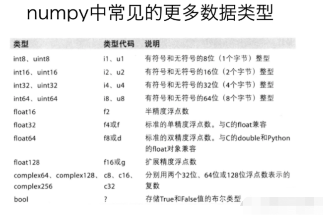
3. Data type operation:

3.1. Specify the data type of the created array:

a=np.array([1,0,1,0],dtype=np.bool)
# The returned result is shown on the right: [true false]
print a

3.2. Modify the data type of the array:

a = np.array([1, 0, 1, 0], dtype=np.bool)
a=a.astype(np.float)
# The returned result is shown on the right: [1. 0. 1. 0.]
print a

3.3. Modify the decimal places of floating-point type:

b = np.array([0.1214, 0.1767, 0.1999])
b = np.round(b, 2)
# The returned result is shown on the right: [0.12 0.18 0.2]
print b

4. View the shape of the array

a=np.array([[3,4,5,6,7,8],[4,5,6,7,8,9]])
# The operation results are shown on the right: (2, 6)
print a.shape

5. Modify the shape of the array:

a = np.array([[3, 4, 5, 6, 7, 8], [4, 5, 6, 7, 8, 9]])
a = a.reshape(3, 4)
# The operation results are shown on the right: (3, 4)
print a.shape

6. Convert the array into one-dimensional data:

a = np.array([[3, 4, 5, 6, 7, 8], [4, 5, 6, 7, 8, 9]])
a = a.reshape(1, 12)
# The operation result is shown on the right: [3 4 5 6 7 8 4 5 6 7 8 9]
print a.flatten()

7. Numpy index and slice:

a = np.array([
    [0, 1, 2, 3],
    [4, 5, 6, 7],
    [8, 9, 10, 11]])
# Take a line, [4 5 6 7]
print a[1]

# Take a column, [2 6 10]
print a[:, 2]

# Take multiple lines, [[4 5 6 7]
#        [ 8  9 10 11]]
print a[1:3]

# Take multiple columns, [[2, 3]
#         [ 6  7]
#         [10 11]]
print a[:, 2:4]

# Take some rows, all columns, [[4 5 6 7]
#                 [ 8  9 10 11]]
print a[[1, 2], :]

# Take all rows, some columns, [[2, 3]
#                  [ 6  7]
#                  [10 11]]
print a[:, [2, 3]]

8. Boolean index in numpy:

t = np.arange(24).reshape((4, 6))
# Change the value of t value less than 10 to 0
t[t < 10] = 0
print t
# The operation results are as follows:
# [[0  0  0  0  0  0]
#  [0  0  0  0 10 11]
# [12 13 14 15 16 17]
# [18 19 20 21 22 23]]

9. Ternary operator in numpy:

t = np.arange(24).reshape((4, 6))
# Change the value of t less than 10 to 0, otherwise change it to 10, the ternary operator of numpy
t = np.where(t < 10, 0, 10)
print t
# The operation results are as follows:
'''
[[ 0  0  0  0  0  0]
[ 0  0  0  0 10 10]
[10 10 10 10 10 10]
[10 10 10 10 10 10]]
'''

10. Clip in numpy:

t = np.array([[0, 1, 2, 3, 4, 5],
              [6, 7, 8, 9, 10, 11],
              [12, 13, 14, 15, 16, 17],
              [18, 19, 20, np.nan, np.nan, np.nan]])

# Change the value of t value less than 10 to 10 and greater than or equal to 18 to 18
t = np.clip(t, 10, 18)
print t
# The operation results are as follows:
'''
[[10. 10. 10. 10. 10. 10.]
[10. 10. 10. 10. 10. 11.]
[12. 13. 14. 15. 16. 17.]
[18. 18. 18. nan nan nan]]
'''

11，np.nan and NP inf

nan:not a number means it is not a number. When we read the local file as float, it will appear if it is missing Or as an inappropriate calculation (infinity minus infinity);

Inf represents positive infinity, - inf represents negative infinity;

a=np.inf
#1. The type of infinity is: < type 'float' >
print type(a)

#2. The type of nan is: < type 'float' >
b=np.nan
print type(b)
#3. Two nan are not equal, False
print np.nan == np.nan

#4. Using the above characteristics, you can judge the number of nan in the array, 1
t=np.array([1.,2.,np.nan])
print np.count_nonzero(t != t)

# 5. If the data contains nan, replace it with 0, [1.2.0.]
t[np.isnan(t)]=0
print t

2, ufunc(universal function object) is a general term for functions that process arrays

1. Statistical functions commonly used in numpy

• Summation: t.sum(axis=None)

• Mean: t.mean(a,axis=None)

• Median: NP median(t,axis=None)

• Maximum value: t.max(axis=None)

• Minimum value: t.min(axis=None)

• Extreme value: NP ptp(t,axis=None)

• Standard deviation: t.std(axis=None)

2. Other common methods:

• Get the location of the maximum and minimum values: NP argmax(t,axis=0)  ; np.argmin(t,axis=1)

• Create an array with all 0: NP zeros((3,4))

• Create an array with all 1: NP ones((3,4))

• Create an array with a diagonal of 1: NP eye(3))

 

3. Functions of some random numbers

 

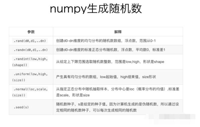
# np.random.rand() the parameter of this function is the dimension of the array, and the value range is [0,1]

# 0.761440624168
print np.random.rand()

# [0.91673038]
print np.random.rand(1)

# [[0.3286804  0.94399189]
#  [0.99691882 0.51908634]]
print np.random.rand(2, 2)

np.random.randn()
np.random.randn(1)
np.random.randn(2, 2)


np.random.randint(1)
np.random.randint(1, 5)
np.random.randint(1, 12, size=(3, 4))


np.random.uniform(1,12,size=(3,4))


np.random.normal(0,1,size=(3,4))