Note:
Click here to download the full example code

Transformer tutorial

Author: Zihao Ye, Jinjing Zhou, Qipeng Guo, Quan Gan, Zheng Zhang
In this tutorial, you will learn a simplified implementation of the Transformer model. You can see the highlights of the most important design points. For example, there is only one head of attention. The complete code can be found in Here Find it.

Overall structure and research papers Annotated Transformer The structure in is similar.

In the research paper, the Transformer model is introduced to replace CNN / RNN architecture for sequence modeling, which is“ Attention is All You Need " It improves machine translation and natural language reasoning tasks( GPT )Technical level. With large corpus( BERT )The latest work of pre training Transformer supports it to learn high quality semantic representation.

The interesting part of transformers is its wide attention. Note that the classic usage comes from the machine translation model, where the output token appears on all input tokens.

The transformer also exerts self-care in the decoder and encoder. Regardless of the position of words in a sequence, this process forces words to be related to each other to be grouped together. This is different from the RNN based model, in which words (in the source sentence) are combined along the chain, which is considered to be too limited.

Attention layer of Transformer

In Transformer's focus layer, the module assigns weights to each node learning on its incoming edge. For node pair (i,j)(i,j)(i,j) (from iii to jjj) and node xi,xj ∈ Rnx I, xj \ in \ mathbb {r} ^ nxi, xj ∈ Rn, their connection fractions are defined as follows:
qj=Wq⋅xjki=Wk⋅xivi=Wv⋅xiscore=qjTkiq_j = W_q\cdot x_j \\ k_i = W_k\cdot x_i\\ v_i = W_v\cdot x_i\\ \textrm{score} = q_j^T k_iqj​=Wq​⋅xj​ki​=Wk​⋅xi​vi​=Wv​⋅xi​score=qjT​ki​
Where Wq,Wk,Wv ∈ Rn × DKW ﹣ Q, w ﹣ K, w ﹣ V \ in \ matchb {r} ^ {n \ times d ﹣ Wq,Wk,Wv ∈ Rn × dk map represents xxx as "query", "key" and "value" spaces respectively.

There are other possibilities for score. The point product can measure the similarity of a given query qjq ﹣ JQJ and a key KIK ﹣ IKI: if j needs the information iii stored in it, the query vector j jjj (qjq ﹣ JQJ) of the location should approach the key vector iii (KIK ﹣ IKI) at the location.

The fraction is then used to calculate the sum of normalized input values wvwwv stored in the weight. Then apply the affine layer to wvwvwv to get the output ooo
wji=exp⁡{scoreji}∑(k,i)∈Eexp⁡{scoreki}wvi=∑(k,i)∈Ewkivko=Wo⋅wvw_{ji} = \frac{\exp\{\textrm{score}_{ji} \}}{\sum\limits_{(k, i)\in E}\exp\{\textrm{score}_{ki} \}} \\ \textrm{wv}_i = \sum_{(k, i)\in E} w_{ki} v_k \\ o = W_o\cdot \textrm{wv}wji​=(k,i)∈E∑​exp{scoreki​}exp{scoreji​}​wvi​=(k,i)∈E∑​wki​vk​o=Wo​⋅wv

Multi-head attention layer

In transformers, attention is multi headed. The head is very much like a channel in a convolutional network. Multiple attention consists of multiple attention heads, each of which refers to an attention module. wv(i)wv^{(i)}wv(i) all headers are concatenated and mapped to the output o affine layer:
o=Wo⋅concat([wv(0),wv(1),⋯ ,wv(h)])o = W_o \cdot \textrm{concat}\left(\left[\textrm{wv}^{(0)}, \textrm{wv}^{(1)}, \cdots, \textrm{wv}^{(h)}\right]\right)o=Wo​⋅concat([wv(0),wv(1),⋯,wv(h)])
The following code wraps the necessary components for multi headed attention and provides two interfaces.

• get maps the status "x" to queries, keys, and values, which are required in the next step (propagate? Attention).
• Get o maps the updated values after focus to the output ooo for post-processing.

class MultiHeadAttention(nn.Module):
    "Multi-Head Attention"
    def __init__(self, h, dim_model):
        "h: number of heads; dim_model: hidden dimension"
        super(MultiHeadAttention, self).__init__()
        self.d_k = dim_model // h
        self.h = h
        # W_q, W_k, W_v, W_o
        self.linears = clones(nn.Linear(dim_model, dim_model), 4)

    def get(self, x, fields='qkv'):
        "Return a dict of queries / keys / values."
        batch_size = x.shape[0]
        ret = {}
        if 'q' in fields:
            ret['q'] = self.linears[0](x).view(batch_size, self.h, self.d_k)
        if 'k' in fields:
            ret['k'] = self.linears[1](x).view(batch_size, self.h, self.d_k)
        if 'v' in fields:
            ret['v'] = self.linears[2](x).view(batch_size, self.h, self.d_k)
        return ret

    def get_o(self, x):
        "get output of the multi-head attention"
        batch_size = x.shape[0]
        return self.linears[3](x.view(batch_size, -1))

How DGL implements Transformer with a graph neural network

You get a different perspective from Transformer by treating attention as an edge in the graph and initiating appropriate processing with messages delivered on the edge.

Graph structure

The graph is constructed by mapping the tags of source and target sentences to nodes. The complete Transformer diagram consists of three subgraphs:

Source language map. This is a complete graph, and each token si can participate in any other token sj (including self loop).

Target language map. The graph is semi complete because ti only participates in tj if I > J (the output token cannot depend on future words).

Cross language map. This is a two-way graph in which each source token has an edge si and each target Token tj, which means that each target token can participate in the source token.

The complete picture is as follows:

Pre build the drawing in the data set preparation phase.

Message passing

After defining the graph structure, continue to define calculations for messaging.

Suppose you have calculated all queries, keys, and values. For each node iii (whether it is a source token or a target Token), you can divide attention calculation into two steps:

• Message calculation: calculate the attention score between scoreijscore {ij} scoreij and all nodes jjj participate in Qiq} and KJK} jkj through scaling point product between participants. The email sent from jjj to iii will be composed of scoreijscore {ij} scoreij and value vjv {jvj.
• Message aggregation: the aggregation value vjv_jvj comes from all jjj according to the score scoreijscore {ij} scoreij.

Simple implementation

Message computation

Calculate the v alue of the score source node and send it to the target mailbox

def message_func(edges):
    return {'score': ((edges.src['k'] * edges.dst['q'])
                      .sum(-1, keepdim=True)),
            'v': edges.src['v']}

Message aggregation

Normalize all edges and weighted sums to get output

import torch as th
import torch.nn.functional as F

def reduce_func(nodes, d_k=64):
    v = nodes.mailbox['v']
    att = F.softmax(nodes.mailbox['score'] / th.sqrt(d_k), 1)
    return {'dx': (att * v).sum(1)}

Execute on specific edges

import functools.partial as partial
def naive_propagate_attention(self, g, eids):
    g.send_and_recv(eids, message_func, partial(reduce_func, d_k=self.d_k))

Speeding up with built-in functions

To speed up the messaging process, use DGL's built-in features, including:

• Fn.src ABCD egdes (SRC field, edges field, out field) multiplies the source attribute and edges attribute, and then sends the result to the mailbox out field of the target node whose key is the key.
• Fn.copy (edges field, out field) copies the attributes of edge to the mailbox of the target node
• Fn.sum (edges field, out field) summarizes the attributes of the edge and sends the aggregation to the mailbox of the target node.

Here, you assemble these built-in functions as propagate? Attention, which is also the main graphic operation function in the final implementation. To speed it up, divide the softmax operation into the following steps. Recall that each person in charge has two stages.

1. Calculation of attention fraction qqq by multiplying kkk of src node and dst node

• g.apply_edges(src_dot_dst('k', 'q', 'score'), eids)

2. Softmax scaled on the incoming edge of all dst nodes

Step 1: index using scale normalization constant

• g.apply_edges(scaled_exp('score', np.sqrt(self.d_k)))
  scoreij←exp⁡(scoreijdk)\textrm{score}_{ij}\leftarrow\exp{\left(\frac{\textrm{score}_{ij}}{ \sqrt{d_k}}\right)}scoreij​←exp(dk​​scoreij​​)

Step 2: get the value on the associated node and weighted by the score on the incoming edge of each node; get the sum of the scores on the incoming edge of each node for standardization. Note that wv\textrm{wv}wv is not standardized here.

• msg: fn.src_mul_edge('v', 'score', 'v'), reduce: fn.sum('v', 'wv')
  wvj=∑i=1Nscoreij⋅vi\textrm{wv}_j=\sum_{i=1}^{N} \textrm{score}_{ij} \cdot v_iwvj​=i=1∑N​scoreij​⋅vi​
• msg: fn.copy_edge('score', 'score'), reduce: fn.sum('score', 'z')
  zj=∑i=1Nscoreij\textrm{z}_j=\sum_{i=1}^{N} \textrm{score}_{ij}zj​=i=1∑N​scoreij​
  Normalized wv\textrm{wv}wv is left for later processing.

def src_dot_dst(src_field, dst_field, out_field):
    def func(edges):
        return {out_field: (edges.src[src_field] * edges.dst[dst_field]).sum(-1, keepdim=True)}

    return func

def scaled_exp(field, scale_constant):
    def func(edges):
        # clamp for softmax numerical stability
        return {field: th.exp((edges.data[field] / scale_constant).clamp(-5, 5))}

    return func


def propagate_attention(self, g, eids):
    # Compute attention score
    g.apply_edges(src_dot_dst('k', 'q', 'score'), eids)
    g.apply_edges(scaled_exp('score', np.sqrt(self.d_k)))
    # Update node state
    g.send_and_recv(eids,
                    [fn.src_mul_edge('v', 'score', 'v'), fn.copy_edge('score', 'score')],
                    [fn.sum('v', 'wv'), fn.sum('score', 'z')])

Preprocessing and postprocessing

In Transformer, data needs to be preprocessed before and after the propagate & attention function.
Preprocessing preprocessing function pre func first normalizes node representation, and then maps them to a set of queries, keys and values with self concern as an example:
x←LayerNorm(x)[q,k,v]←[Wq,Wk,Wv]⋅xx \leftarrow \textrm{LayerNorm}(x) \\ [q, k, v] \leftarrow [W_q, W_k, W_v ]\cdot xx←LayerNorm(x)[q,k,v]←[Wq​,Wk​,Wv​]⋅x
The post-processing functions complete the whole calculation corresponding to the first layer of transformer: 1. Normalize the wv and obtain the output o of multi-channel attention layer.
wv←wvzo←Wo⋅wv+bo\textrm{wv} \leftarrow \frac{\textrm{wv}}{z} \\ o \leftarrow W_o\cdot \textrm{wv} + b_owv←zwv​o←Wo​⋅wv+bo​
Add remaining connections:
x←x+ox \leftarrow x + ox←x+o
2. Apply two layers of position feed-forward layer xxx on it and then add the remaining connections:
x←x+LayerNorm(FFN(x))x \leftarrow x + \textrm{LayerNorm}(\textrm{FFN}(x))x←x+LayerNorm(FFN(x))
Where ffnffnfn refers to feedforward function.

class Encoder(nn.Module):
    def __init__(self, layer, N):
        super(Encoder, self).__init__()
        self.N = N
        self.layers = clones(layer, N)
        self.norm = LayerNorm(layer.size)

    def pre_func(self, i, fields='qkv'):
        layer = self.layers[i]
        def func(nodes):
            x = nodes.data['x']
            norm_x = layer.sublayer[0].norm(x)
            return layer.self_attn.get(norm_x, fields=fields)
        return func

    def post_func(self, i):
        layer = self.layers[i]
        def func(nodes):
            x, wv, z = nodes.data['x'], nodes.data['wv'], nodes.data['z']
            o = layer.self_attn.get_o(wv / z)
            x = x + layer.sublayer[0].dropout(o)
            x = layer.sublayer[1](x, layer.feed_forward)
            return {'x': x if i < self.N - 1 else self.norm(x)}
        return func

class Decoder(nn.Module):
    def __init__(self, layer, N):
        super(Decoder, self).__init__()
        self.N = N
        self.layers = clones(layer, N)
        self.norm = LayerNorm(layer.size)

    def pre_func(self, i, fields='qkv', l=0):
        layer = self.layers[i]
        def func(nodes):
            x = nodes.data['x']
            if fields == 'kv':
                norm_x = x # In enc-dec attention, x has already been normalized.
            else:
                norm_x = layer.sublayer[l].norm(x)
            return layer.self_attn.get(norm_x, fields)
        return func

    def post_func(self, i, l=0):
        layer = self.layers[i]
        def func(nodes):
            x, wv, z = nodes.data['x'], nodes.data['wv'], nodes.data['z']
            o = layer.self_attn.get_o(wv / z)
            x = x + layer.sublayer[l].dropout(o)
            if l == 1:
                x = layer.sublayer[2](x, layer.feed_forward)
            return {'x': x if i < self.N - 1 else self.norm(x)}
        return func

In this way, all the processes of one layer encoder and decoder in Transformer are completed.

Main class of Transformer graph

You can think of the Transformer's processing flow as two-stage message passing (pre-processing and post-processing are added appropriately) in a complete graph: 1) self attention in the encoder, 2) self attention in the decoder, and then cross the attention between the encoder and the decoder, as shown below.

class Transformer(nn.Module):
    def __init__(self, encoder, decoder, src_embed, tgt_embed, pos_enc, generator, h, d_k):
        super(Transformer, self).__init__()
        self.encoder, self.decoder = encoder, decoder
        self.src_embed, self.tgt_embed = src_embed, tgt_embed
        self.pos_enc = pos_enc
        self.generator = generator
        self.h, self.d_k = h, d_k

    def propagate_attention(self, g, eids):
        # Compute attention score
        g.apply_edges(src_dot_dst('k', 'q', 'score'), eids)
        g.apply_edges(scaled_exp('score', np.sqrt(self.d_k)))
        # Send weighted values to target nodes
        g.send_and_recv(eids,
                        [fn.src_mul_edge('v', 'score', 'v'), fn.copy_edge('score', 'score')],
                        [fn.sum('v', 'wv'), fn.sum('score', 'z')])

    def update_graph(self, g, eids, pre_pairs, post_pairs):
        "Update the node states and edge states of the graph."

        # Pre-compute queries and key-value pairs.
        for pre_func, nids in pre_pairs:
            g.apply_nodes(pre_func, nids)
        self.propagate_attention(g, eids)
        # Further calculation after attention mechanism
        for post_func, nids in post_pairs:
            g.apply_nodes(post_func, nids)

    def forward(self, graph):
        g = graph.g
        nids, eids = graph.nids, graph.eids

        # Word Embedding and Position Embedding
        src_embed, src_pos = self.src_embed(graph.src[0]), self.pos_enc(graph.src[1])
        tgt_embed, tgt_pos = self.tgt_embed(graph.tgt[0]), self.pos_enc(graph.tgt[1])
        g.nodes[nids['enc']].data['x'] = self.pos_enc.dropout(src_embed + src_pos)
        g.nodes[nids['dec']].data['x'] = self.pos_enc.dropout(tgt_embed + tgt_pos)

        for i in range(self.encoder.N):
            # Step 1: Encoder Self-attention
            pre_func = self.encoder.pre_func(i, 'qkv')
            post_func = self.encoder.post_func(i)
            nodes, edges = nids['enc'], eids['ee']
            self.update_graph(g, edges, [(pre_func, nodes)], [(post_func, nodes)])

        for i in range(self.decoder.N):
            # Step 2: Dncoder Self-attention
            pre_func = self.decoder.pre_func(i, 'qkv')
            post_func = self.decoder.post_func(i)
            nodes, edges = nids['dec'], eids['dd']
            self.update_graph(g, edges, [(pre_func, nodes)], [(post_func, nodes)])
            # Step 3: Encoder-Decoder attention
            pre_q = self.decoder.pre_func(i, 'q', 1)
            pre_kv = self.decoder.pre_func(i, 'kv', 1)
            post_func = self.decoder.post_func(i, 1)
            nodes_e, nodes_d, edges = nids['enc'], nids['dec'], eids['ed']
            self.update_graph(g, edges, [(pre_q, nodes_d), (pre_kv, nodes_e)], [(post_func, nodes_d)])

        return self.generator(g.ndata['x'][nids['dec']])

Training

This tutorial does not cover other techniques, such as tag smoothing and Noam optimization mentioned in the original paper. For a detailed description of these modules, read the Annotated transformer.

Task and the dataset

Transformer is a general framework for various NLP tasks. This tutorial focuses on sequence learning: This is a typical example of how it works.

For datasets, there are two example tasks: copy and sort, and two actual translation tasks: the multi30k en de task and the wmt14 en de task.

• Copy dataset: copies the input sequence to the output. (training / effective / test: 9000, 1000, 1000)
• Sort dataset: sorts the input sequence to output. (training / effective / test: 9000, 1000, 1000)
• Multi30k En De, which converts sentences from En to de. (training / effective / test: 29000, 1000, 1000)
• Wmt14 En De, translating sentences from En to de. (training / effective / test: 4500966 / 3000 / 3003)

Graph building

Batch processing is similar to the way you work with tree LSTM. Build a graph pool in advance, including all possible combinations of input length and output length. Then, for each sample in the batch, the batch graph of dgl.batch's size is called as a large graph together.
You can wrap the process of creating a graph pool and building a BatchedGraph in dataset.GraphPool and dataset.TranslationDataset.

graph_pool = GraphPool()

data_iter = dataset(graph_pool, mode='train', batch_size=1, devices=devices)
for graph in data_iter:
    print(graph.nids['enc']) # encoder node ids
    print(graph.nids['dec']) # decoder node ids
    print(graph.eids['ee']) # encoder-encoder edge ids
    print(graph.eids['ed']) # encoder-decoder edge ids
    print(graph.eids['dd']) # decoder-decoder edge ids
    print(graph.src[0]) # Input word index list
    print(graph.src[1]) # Input positions
    print(graph.tgt[0]) # Output word index list
    print(graph.tgt[1]) # Ouptut positions
    break

out:

tensor([0, 1, 2, 3, 4, 5, 6, 7, 8], device='cuda:0')
tensor([ 9, 10, 11, 12, 13, 14, 15, 16, 17, 18], device='cuda:0')
tensor([ 0,  1,  2,  3,  4,  5,  6,  7,  8,  9, 10, 11, 12, 13, 14, 15, 16, 17,
        18, 19, 20, 21, 22, 23, 24, 25, 26, 27, 28, 29, 30, 31, 32, 33, 34, 35,
        36, 37, 38, 39, 40, 41, 42, 43, 44, 45, 46, 47, 48, 49, 50, 51, 52, 53,
        54, 55, 56, 57, 58, 59, 60, 61, 62, 63, 64, 65, 66, 67, 68, 69, 70, 71,
        72, 73, 74, 75, 76, 77, 78, 79, 80], device='cuda:0')
tensor([ 81,  82,  83,  84,  85,  86,  87,  88,  89,  90,  91,  92,  93,  94,
         95,  96,  97,  98,  99, 100, 101, 102, 103, 104, 105, 106, 107, 108,
        109, 110, 111, 112, 113, 114, 115, 116, 117, 118, 119, 120, 121, 122,
        123, 124, 125, 126, 127, 128, 129, 130, 131, 132, 133, 134, 135, 136,
        137, 138, 139, 140, 141, 142, 143, 144, 145, 146, 147, 148, 149, 150,
        151, 152, 153, 154, 155, 156, 157, 158, 159, 160, 161, 162, 163, 164,
        165, 166, 167, 168, 169, 170], device='cuda:0')
tensor([171, 172, 173, 174, 175, 176, 177, 178, 179, 180, 181, 182, 183, 184,
        185, 186, 187, 188, 189, 190, 191, 192, 193, 194, 195, 196, 197, 198,
        199, 200, 201, 202, 203, 204, 205, 206, 207, 208, 209, 210, 211, 212,
        213, 214, 215, 216, 217, 218, 219, 220, 221, 222, 223, 224, 225],
       device='cuda:0')
tensor([28, 25,  7, 26,  6,  4,  5,  9, 18], device='cuda:0')
tensor([0, 1, 2, 3, 4, 5, 6, 7, 8], device='cuda:0')
tensor([ 0, 28, 25,  7, 26,  6,  4,  5,  9, 18], device='cuda:0')
tensor([0, 1, 2, 3, 4, 5, 6, 7, 8, 9], device='cuda:0')

Put it all together

Train a layer of 128 size single head transformer on the replication task. Set other parameters to default values.

The inference module is not included in this tutorial. It requires a beam search. For a complete implementation, see GitHub repo.

from tqdm import tqdm
import torch as th
import numpy as np

from loss import LabelSmoothing, SimpleLossCompute
from modules import make_model
from optims import NoamOpt
from dgl.contrib.transformer import get_dataset, GraphPool

def run_epoch(data_iter, model, loss_compute, is_train=True):
    for i, g in tqdm(enumerate(data_iter)):
        with th.set_grad_enabled(is_train):
            output = model(g)
            loss = loss_compute(output, g.tgt_y, g.n_tokens)
    print('average loss: {}'.format(loss_compute.avg_loss))
    print('accuracy: {}'.format(loss_compute.accuracy))

N = 1
batch_size = 128
devices = ['cuda' if th.cuda.is_available() else 'cpu']

dataset = get_dataset("copy")
V = dataset.vocab_size
criterion = LabelSmoothing(V, padding_idx=dataset.pad_id, smoothing=0.1)
dim_model = 128

# Create model
model = make_model(V, V, N=N, dim_model=128, dim_ff=128, h=1)

# Sharing weights between Encoder & Decoder
model.src_embed.lut.weight = model.tgt_embed.lut.weight
model.generator.proj.weight = model.tgt_embed.lut.weight

model, criterion = model.to(devices[0]), criterion.to(devices[0])
model_opt = NoamOpt(dim_model, 1, 400,
                    th.optim.Adam(model.parameters(), lr=1e-3, betas=(0.9, 0.98), eps=1e-9))
loss_compute = SimpleLossCompute

att_maps = []
for epoch in range(4):
    train_iter = dataset(graph_pool, mode='train', batch_size=batch_size, devices=devices)
    valid_iter = dataset(graph_pool, mode='valid', batch_size=batch_size, devices=devices)
    print('Epoch: {} Training...'.format(epoch))
    model.train(True)
    run_epoch(train_iter, model,
              loss_compute(criterion, model_opt), is_train=True)
    print('Epoch: {} Evaluating...'.format(epoch))
    model.att_weight_map = None
    model.eval()
    run_epoch(valid_iter, model,
              loss_compute(criterion, None), is_train=False)
    att_maps.append(model.att_weight_map)

Visualization

After training, you can visualize the attention Transformer generates on the replication task.

src_seq = dataset.get_seq_by_id(VIZ_IDX, mode='valid', field='src')
tgt_seq = dataset.get_seq_by_id(VIZ_IDX, mode='valid', field='tgt')[:-1]
# visualize head 0 of encoder-decoder attention
att_animation(att_maps, 'e2d', src_seq, tgt_seq, 0)

As can be seen from the figure, decoder nodes gradually learn to participate in the corresponding nodes according to the input order, which is the expected behavior.

Multi-head attention

In addition to single head attention training, which focuses on playing tasks. We also visualize the self attention of the encoder, the self attention of the decoder and the attention score of the encoder decoder in a single-layer transformer network trained on multiple 30k datasets.

From the visualization, you can see the diversity of different heads. Different minds learn different relationships between pairs of words.

• Encoder self attention

• Encoder decoder note that most of the words in the target sequence are related to their related words in the source sequence, for example, when generating "See" (in De), multiple headers are on "lake"; when generating "Eisfischerh ü tte", several principals participate in "ice".

• Self attention of decoder most words appear with the first few words.

Adaptive Universal Transformer

Google's recently published research paper Universal Transformer is an example of how update graph can adapt to more complex update rules.

The purpose of general Transformer is to solve the problem that vanilla Transformer is not general in calculation by introducing recurrence in Transformer

• The basic idea of Universal Transformer is to repeatedly modify the representation of all symbols in the sequence by applying a Transformer layer to the representation in each repeating step.
• Compared with normal Transformer, Universal Transformer shares the weight among its layers, and it does not fix the repetition time (which means the number of layers in Transformer).

Further optimization and adoption Adaptive computation time (ACT) Mechanism to allow the model to dynamically adjust the number of times the representation of each position in the sequence has been modified (hereafter referred to as a step). This model is also called adaptive universal transformer (AUT).

In AUT, you maintain a list of active nodes. At each step of ttt, we calculate the probability of stopping: H (0 < h < 1) H (0 < h < 1) H (0 < h < 1) for all nodes in this list, by:
hit=σ(Whxit+bh)h^t_i = \sigma(W_h x^t_i + b_h)hit​=σ(Wh​xit​+bh​)
It then dynamically determines which nodes are still active. A node pauses t t t only if ∑ t=1T − 1ht < 1 − ε ≤∑ t = 1tht \ sum {t = 1} ^ {T-1} h {t} h ∑ t=1T − 1 ht < 1 − ε t ≤Σ t=1T ht. The paused node is removed from the list. The process continues until the list is empty or the predefined maximum steps are reached. From a DGL perspective, this means that the activity graph becomes sparse over time.

The final state of the node is the weighted average value of xtix through htih ^ {I} HTI:
si=∑t=1Thit⋅xits_i = \sum_{t=1}^{T} h_i^t\cdot x_i^tsi​=t=1∑T​hit​⋅xit​
In DGL, the algorithm is implemented by calling the node whose update graph is still active and the edge associated with this node. The following code shows the Universal Transformer class in DGL:

class UTransformer(nn.Module):
    "Universal Transformer(https://arxiv.org/pdf/1807.03819.pdf) with ACT(https://arxiv.org/pdf/1603.08983.pdf)."
    MAX_DEPTH = 8
    thres = 0.99
    act_loss_weight = 0.01
    def __init__(self, encoder, decoder, src_embed, tgt_embed, pos_enc, time_enc, generator, h, d_k):
        super(UTransformer, self).__init__()
        self.encoder,  self.decoder = encoder, decoder
        self.src_embed, self.tgt_embed = src_embed, tgt_embed
        self.pos_enc, self.time_enc = pos_enc, time_enc
        self.halt_enc = HaltingUnit(h * d_k)
        self.halt_dec = HaltingUnit(h * d_k)
        self.generator = generator
        self.h, self.d_k = h, d_k

    def step_forward(self, nodes):
        # add positional encoding and time encoding, increment step by one
        x = nodes.data['x']
        step = nodes.data['step']
        pos = nodes.data['pos']
        return {'x': self.pos_enc.dropout(x + self.pos_enc(pos.view(-1)) + self.time_enc(step.view(-1))),
                'step': step + 1}

    def halt_and_accum(self, name, end=False):
        "field: 'enc' or 'dec'"
        halt = self.halt_enc if name == 'enc' else self.halt_dec
        thres = self.thres
        def func(nodes):
            p = halt(nodes.data['x'])
            sum_p = nodes.data['sum_p'] + p
            active = (sum_p < thres) & (1 - end)
            _continue = active.float()
            r = nodes.data['r'] * (1 - _continue) + (1 - sum_p) * _continue
            s = nodes.data['s'] + ((1 - _continue) * r + _continue * p) * nodes.data['x']
            return {'p': p, 'sum_p': sum_p, 'r': r, 's': s, 'active': active}
        return func

    def propagate_attention(self, g, eids):
        # Compute attention score
        g.apply_edges(src_dot_dst('k', 'q', 'score'), eids)
        g.apply_edges(scaled_exp('score', np.sqrt(self.d_k)), eids)
        # Send weighted values to target nodes
        g.send_and_recv(eids,
                        [fn.src_mul_edge('v', 'score', 'v'), fn.copy_edge('score', 'score')],
                        [fn.sum('v', 'wv'), fn.sum('score', 'z')])

    def update_graph(self, g, eids, pre_pairs, post_pairs):
        "Update the node states and edge states of the graph."
        # Pre-compute queries and key-value pairs.
        for pre_func, nids in pre_pairs:
            g.apply_nodes(pre_func, nids)
        self.propagate_attention(g, eids)
        # Further calculation after attention mechanism
        for post_func, nids in post_pairs:
            g.apply_nodes(post_func, nids)

    def forward(self, graph):
        g = graph.g
        N, E = graph.n_nodes, graph.n_edges
        nids, eids = graph.nids, graph.eids

        # embed & pos
        g.nodes[nids['enc']].data['x'] = self.src_embed(graph.src[0])
        g.nodes[nids['dec']].data['x'] = self.tgt_embed(graph.tgt[0])
        g.nodes[nids['enc']].data['pos'] = graph.src[1]
        g.nodes[nids['dec']].data['pos'] = graph.tgt[1]

        # init step
        device = next(self.parameters()).device
        g.ndata['s'] = th.zeros(N, self.h * self.d_k, dtype=th.float, device=device)    # accumulated state
        g.ndata['p'] = th.zeros(N, 1, dtype=th.float, device=device)                    # halting prob
        g.ndata['r'] = th.ones(N, 1, dtype=th.float, device=device)                     # remainder
        g.ndata['sum_p'] = th.zeros(N, 1, dtype=th.float, device=device)                # sum of pondering values
        g.ndata['step'] = th.zeros(N, 1, dtype=th.long, device=device)                  # step
        g.ndata['active'] = th.ones(N, 1, dtype=th.uint8, device=device)                # active

        for step in range(self.MAX_DEPTH):
            pre_func = self.encoder.pre_func('qkv')
            post_func = self.encoder.post_func()
            nodes = g.filter_nodes(lambda v: v.data['active'].view(-1), nids['enc'])
            if len(nodes) == 0: break
            edges = g.filter_edges(lambda e: e.dst['active'].view(-1), eids['ee'])
            end = step == self.MAX_DEPTH - 1
            self.update_graph(g, edges,
                              [(self.step_forward, nodes), (pre_func, nodes)],
                              [(post_func, nodes), (self.halt_and_accum('enc', end), nodes)])

        g.nodes[nids['enc']].data['x'] = self.encoder.norm(g.nodes[nids['enc']].data['s'])

        for step in range(self.MAX_DEPTH):
            pre_func = self.decoder.pre_func('qkv')
            post_func = self.decoder.post_func()
            nodes = g.filter_nodes(lambda v: v.data['active'].view(-1), nids['dec'])
            if len(nodes) == 0: break
            edges = g.filter_edges(lambda e: e.dst['active'].view(-1), eids['dd'])
            self.update_graph(g, edges,
                              [(self.step_forward, nodes), (pre_func, nodes)],
                              [(post_func, nodes)])

            pre_q = self.decoder.pre_func('q', 1)
            pre_kv = self.decoder.pre_func('kv', 1)
            post_func = self.decoder.post_func(1)
            nodes_e = nids['enc']
            edges = g.filter_edges(lambda e: e.dst['active'].view(-1), eids['ed'])
            end = step == self.MAX_DEPTH - 1
            self.update_graph(g, edges,
                              [(pre_q, nodes), (pre_kv, nodes_e)],
                              [(post_func, nodes), (self.halt_and_accum('dec', end), nodes)])

        g.nodes[nids['dec']].data['x'] = self.decoder.norm(g.nodes[nids['dec']].data['s'])
        act_loss = th.mean(g.ndata['r']) # ACT loss

        return self.generator(g.ndata['x'][nids['dec']]), act_loss * self.act_loss_weight

Call Filter > nodes and Filter > edge to find the node / edge that is still active:

Note:

• filter_nodes() Combine predicates and nodes ID list/Tensor as input, then returns the node satisfying the given predicate ID Tensors.
• filter_edges() Accept predicates and edges ID list/Tensor as input, then returns the edge that satisfies the given predicate ID Tensors.

For a complete implementation, see GitHub repo.

The following illustration shows the effect of adaptive calculation time. Different positions of sentences are revised at different times.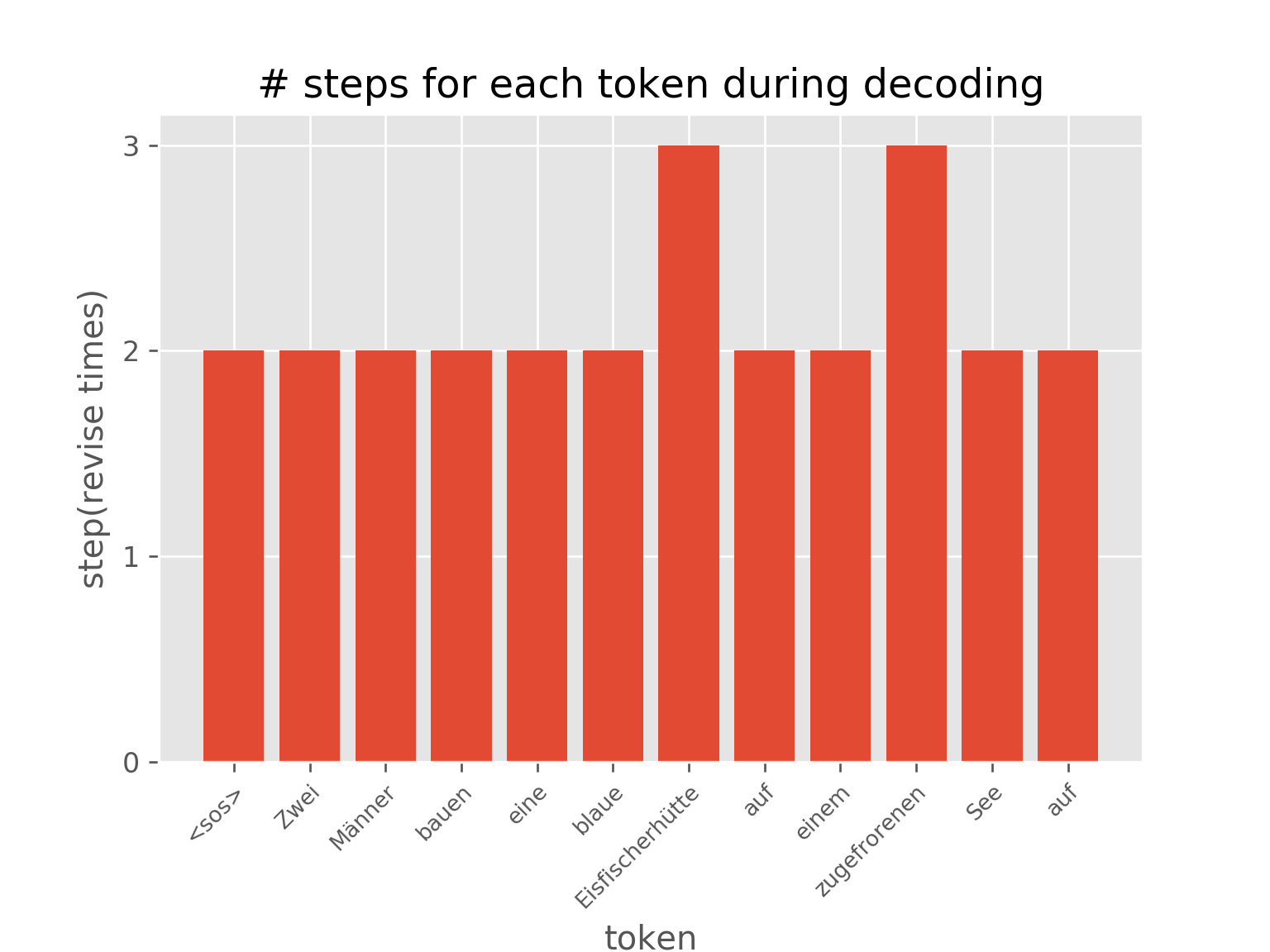

You can also visualize the dynamic step distribution on the nodes during the AUT training of sorting tasks (with an accuracy of 99.7%), which demonstrates how AUT can learn to reduce repetitive steps in training.

Total run time of script: (0 minutes 0.063 seconds)