neuron

   the most basic concept in deep learning: neuron, the popular neural network, is almost composed of neurons combined in different ways. A complete neuron is mainly composed of two parts, namely linear function and excitation function.
   linear function:
     y = wX + b
      the formulas of linear functions are expressed in this way, where x represents input, y represents output, w represents weight and b represents deviation.
     input: the data before neuron processing, x is not necessarily a number, but also a matrix or other data
     output: the data processed by neurons. The output data can also be data in various forms, which is determined by the input data and neurons
     weight: the data multiplied when entering the neuron can be either a number or a matrix. Generally, the initial weight is set randomly. After training, the computer will adjust the weight and assign a larger weight to the relatively important features, while on the contrary, assign a smaller weight to the unimportant features.
     deviation: the linear component is added to the result of multiplying the input and weight, and the linear range can be increased
   activation function (excitation function):
     activation function is to add nonlinear factors to neurons. Because the content that linear function can express has great limitations, many problems in reality are nonlinear, so adding nonlinear factors can increase the fitting effect of the model.

Common activation functions:
  commonly used activation functions include sigmoid function, relu function, tanh function, softmax function, etc.

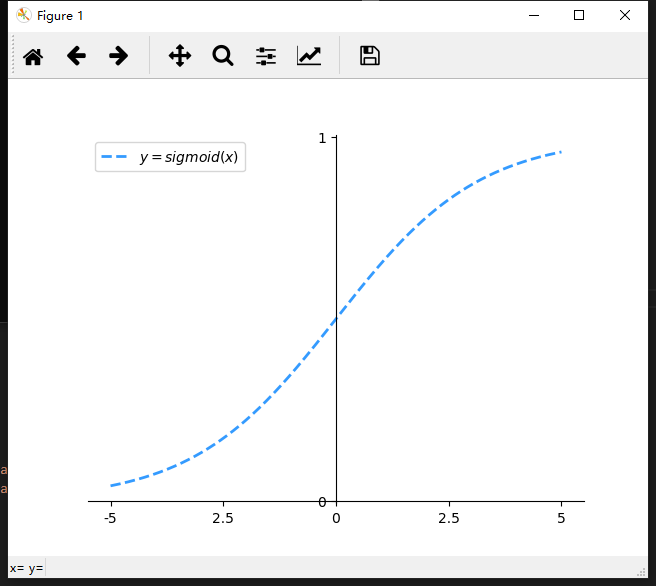
sigmoid function:

   , also known as Logistic function, is used for hidden layer neuron output. The value range is (0,1). It can map a real number to the interval of (0,1) and can be used for binary classification. The effect is better when the feature difference is complex or the difference is not particularly large.
   sigmoid disadvantages: the activation function has a large amount of calculation. When calculating the error gradient by back propagation, the derivation involves division. During back propagation, the gradient will easily disappear, so it is impossible to complete the training of deep network.

   why the gradient disappears: in the back propagation algorithm, the derivation of the activation function is required. The derivative expression of sigmoid is:

   sigmoid original function and derivative graph are as follows: it can be seen from the figure that the derivative quickly approaches 0 from 0, which is easy to cause the phenomenon of "gradient disappearance"

   draw sigmoid function:

"""
Draw a line sigmoid curve
"""
import numpy as np
import matplotlib.pyplot as mp
import math

def sigmoid(x):
    y = 1 / (1 + np.exp(-x))
    return y

# [- π, π] dismantle 1000 points
x = np.linspace(-np.pi, np.pi, 1000)
sigmoid_x = sigmoid(x)

# mapping
mp.plot(x, sigmoid_x, linestyle='--', linewidth=2, 
		color='dodgerblue', alpha=0.9,
		label=r'$y=sigmoid(x)$')

# Modify coordinate scale
x_val_list=[-np.pi, -np.pi/2, 0, np.pi/2, np.pi]
x_text_list=['-5', '2.5', '0', '2.5', '5']
mp.xticks(x_val_list, x_text_list)
mp.yticks([0, 1], 
	      ['0', '1'])

# Set axis
ax = mp.gca()
ax.spines['top'].set_color('none')
ax.spines['right'].set_color('none')
ax.spines['left'].set_position(('data',0))
ax.spines['bottom'].set_position(('data',0))


# Show Legend 
mp.legend(loc='best')
mp.show()

Relu function:
   draw relu function:

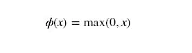
  advantages of ReLU: the convergence speed of SGD obtained with ReLU is much faster than sigmoid/tanh

  the disadvantage of ReLU: it's very "fragile" during training, and it's easy to "die". For example, a very large gradient flows through a ReLU neuron. After updating the parameters, the neuron will no longer activate any data, so the gradient of the neuron will always be 0. If the learning rate is large, it is likely that 40% of the neurons in the network are "dead".

"""
draw relu
"""
import numpy as np
import matplotlib.pyplot as mp
import math

def Relu(x):
    y = []
    for xx in x:
        if xx >= 0:
            y.append(xx)
        else:
            y.append(0)
    return y

# [- π, π] dismantle 1000 points
x = np.linspace(-np.pi, np.pi, 1000)
Relu_x = Relu(x)

# mapping
mp.plot(x, Relu_x, linestyle='--', linewidth=2, 
		color='dodgerblue', alpha=0.9,
		label=r'$y=relu(x)$')

# Modify coordinate scale
x_val_list=[-np.pi, -np.pi/2, 0, np.pi/2, np.pi]
x_text_list=['-π', r'$-\frac{\pi}{2}$', '0', 
			 r'$\frac{π}{2}$', 'π']
mp.xticks(x_val_list, x_text_list)
mp.yticks([-1, -0.5, 0.5, 1], 
	      ['-1', '-0.5', '0.5', '1'])

# Set axis
ax = mp.gca()
ax.spines['top'].set_color('none')
ax.spines['right'].set_color('none')
ax.spines['left'].set_position(('data',0))
ax.spines['bottom'].set_position(('data',0))
# Show Legend 
mp.legend(loc='best')
mp.show()

tanh function
   draw tanh function:

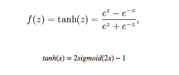
                   8195. The effect of tanh will be very good when the feature difference is obvious, and the feature effect will continue to expand in the process of circulation. The difference between tanh and sigmoid is that tanh is zero mean, so tanh will be better than sigmoid in practical application

"""
Draw a line tanh curve
"""
import numpy as np
import matplotlib.pyplot as mp

# [- π, π] dismantle 1000 points
x = np.linspace(-np.pi, np.pi, 1000)
tanh_x = np.tanh(x)

# mapping
mp.plot(x, tanh_x, linestyle='--', linewidth=2, 
		color='dodgerblue', alpha=0.9,
		label=r'$y=tanh(x)$')

# Modify coordinate scale
x_val_list=[-np.pi, -np.pi/2, 0, np.pi/2, np.pi]
x_text_list=['-π', r'$-\frac{\pi}{2}$', '0', 
			 r'$\frac{π}{2}$', 'π']
mp.xticks(x_val_list, x_text_list)
mp.yticks([-1, -0.5, 0.5, 1], 
	      ['-1', '-0.5', '0.5', '1'])

# Set axis
ax = mp.gca()
ax.spines['top'].set_color('none')
ax.spines['right'].set_color('none')
ax.spines['left'].set_position(('data',0))
ax.spines['bottom'].set_position(('data',0))


# Show Legend 
mp.legend(loc='best')
mp.show()

softmax function

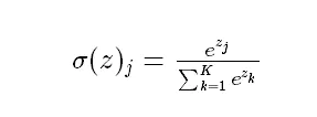
   map the value of the output layer to the 0-1 interval through the activation function, and construct the neuron output into a probability distribution for multi classification problems. The larger the mapping value of the softmax activation function, the greater the possibility of the real category.
   sigmoid is generally used for binary classification problems, while softmax is used for multi classification problems
Reference:
Link: https://www.jianshu.com/p/22d9720dbf1a