1 connectivity

In the image, the smallest unit is the pixel, and there are 8 critical pixels around each pixel. There are three common adjacency relationships: 4 adjacency, 8 adjacency and D adjacency. As shown in the figure below:

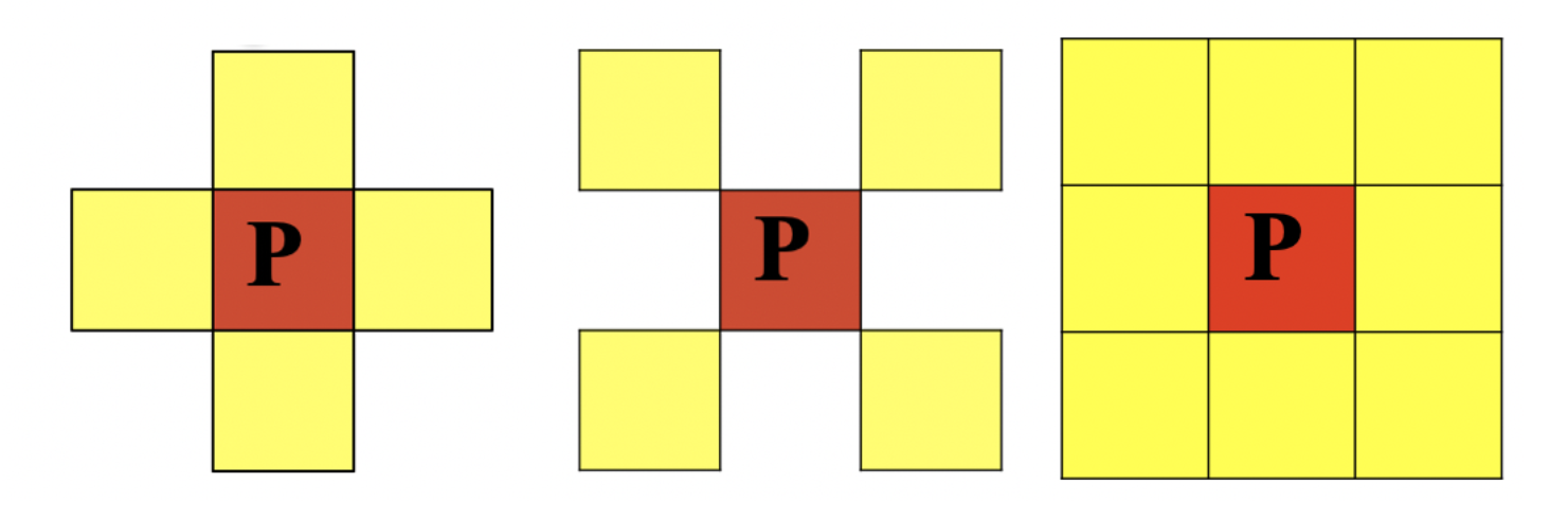
• 4 adjacency: the 4 neighborhood of pixel p (x, y) is: (x+1, y); (x-1，y)； (x，y+1)； (x, y-1), N4 § is used to represent the 4 neighborhood of pixel p
• D adjacency: the D neighborhood of pixel p (x, y) is: the point on the diagonal (x + 1, y + 1); (x+1，y-1)； (x-1，y+1)； (x-1, Y-1), using ND § to represent the D neighborhood of pixel p
• 8 adjacency: the 8 neighborhood of pixel p (x, y) is: the point of 4 neighborhood + the point of D neighborhood, and N8 § is used to represent the 8 neighborhood of pixel p

Connectivity is an important concept for describing regions and boundaries. The two necessary conditions for the connectivity of two pixels are:

1. Are the positions of the two pixels adjacent
2. Whether the gray values of the two pixels meet the specific similarity criteria (or whether they are equal)

According to the definition of connectivity, there are three types: 4 Unicom, 8 Unicom and m Unicom.

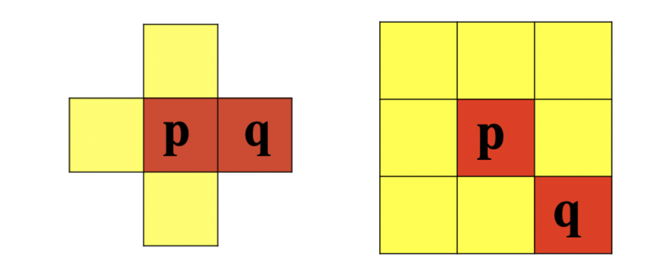
• 4-connected: for pixels p and Q with value V, if q is in set N4 (p), the two pixels are said to be 4-connected

• 8 connectivity: for pixels p and Q with value V, if q is in set N8 (p), the two pixels are said to be 8 connectivity

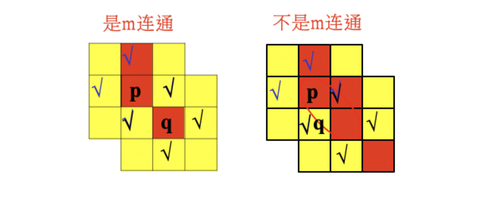
• For pixels p and q with value V, if:

  1. q in set N4 (p), or
  2. Q is in the set ND (p), and the set of N4 (p) and N4(q) is empty (pixels without value V)

  The two pixels are said to be m-connected, that is, the mixed connection of 4-connected and D-connected.

  

2 morphological operation

Morphological transformation is a simple operation based on image shape. It is usually performed on binary images. Corrosion and expansion are two basic morphological operators. Then its variant forms, such as open operation, closed operation, top hat, black hat and so on.

2.1 corrosion and expansion

Corrosion and expansion are the most basic morphological operations. Both corrosion and expansion are for the white part (highlighted part).

Expansion is to expand the highlighted part of the image, and the effect image has a larger highlighted area than the original image; Corrosion is that the highlight area in the original image is eroded, and the effect image has a smaller highlight area than the original image. Expansion is the operation of finding local maximum value, and corrosion is the operation of finding local minimum value.

1. corrosion

   The specific operation is as follows: scan each pixel in the image with A structural element, and operate with each pixel in the structural element and its covered pixel. If they are all 1, the pixel is 1, otherwise it is 0. As shown in the figure below, structure A is corroded by structure B: (the top square in the figure below is wrong!!!)
   

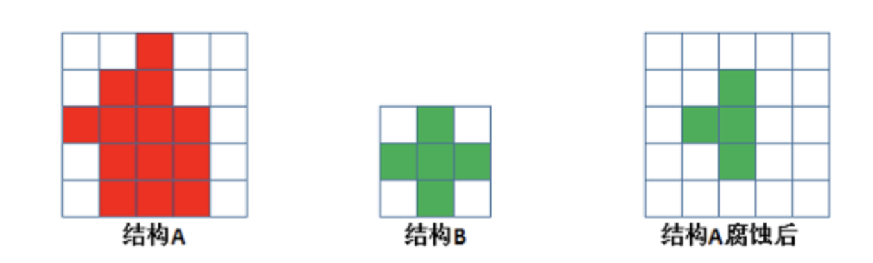
   The function of corrosion is to eliminate the boundary points of the object, reduce the target, and eliminate the noise points smaller than the structural elements.

   API:

   cv.erode(img,kernel,iterations)
   

   Parameters:

   • img: image to process
   • kernel: core structure
   • iterations: the number of times of corrosion. The default value is 1

2. expand

   The specific operation is as follows: scan each pixel in the image with A structural element, and operate with each pixel in the structural element and the pixel covered by it. If they are all 0, the pixel is 0, otherwise it is 1 As shown in the figure below, after structure A is corroded by structure B:

   

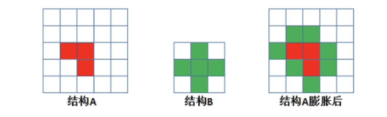
   The function is to combine all the background points in contact with the object into the object to increase the target and supplement the holes in the target.

   API:

   cv.dilate(img,kernel,iterations)
   

   Parameters:

   • img: image to process
   • kernel: core structure
   • iterations: the number of times of corrosion. The default value is 1

   1. Examples

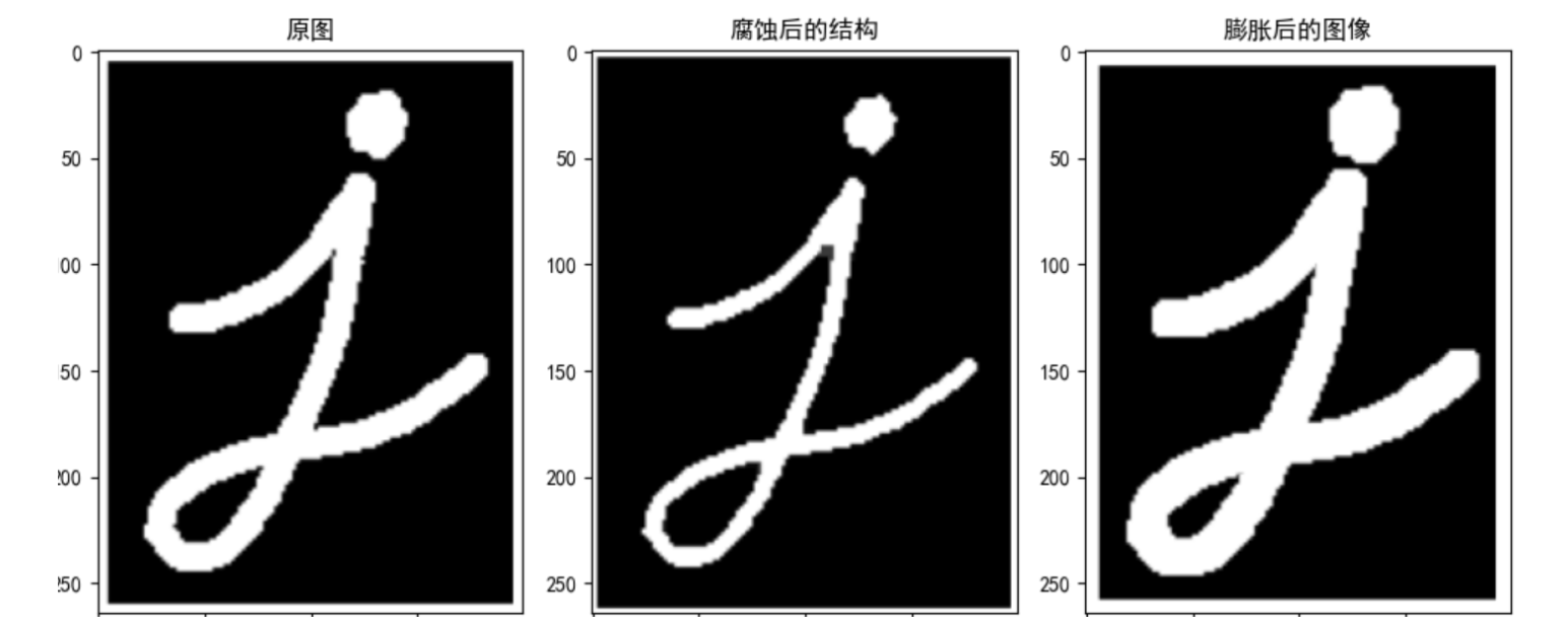
      A 5 * 5 convolution kernel is used to realize the operation of corrosion and expansion:

      import numpy as np
      import cv2 as cv
      import matplotlib.pyplot as plt
      
      # 1 read image
      img = cv.imread("D:\Projects notes\opencv\image\letter.png")
      # 2 create core structure
      kernel = np.ones((5, 5), np.uint8)
      # 3 image corrosion and expansion
      erosion = cv.erode(img, kernel)        # corrosion
      dilate = cv.dilate(img, kernel)        # expand
      # 4 image display
      fig, axes = plt.subplots(nrows=1, ncols=3, figsize=(10, 8), dpi=100)
      axes[0].imshow(img)
      axes[0].set_title("Original drawing")
      axes[1].imshow(erosion)
      axes[1].set_title("Structure after corrosion")
      axes[2].imshow(dilate)
      axes[2].set_title("Expanded image")
      plt.show()
      

2.2 opening and closing operation

Open operation and close operation are to treat corrosion and expansion in a certain order. But the two are not reversible, that is, opening first and then closing can not get the original image.

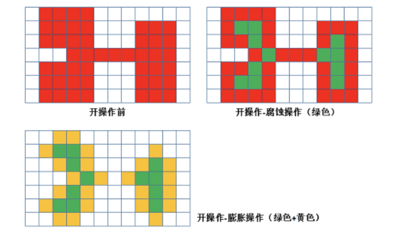
1. Open operation

   The open operation causes corrosion before expansion. Its function is to separate objects and eliminate small areas.

   Features: cook early and remove small interference quickly without affecting the original image.

   

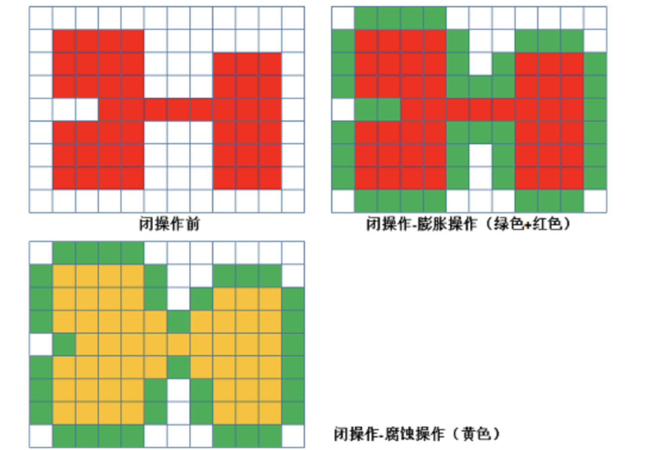
2. Closed operation

   The closed operation is opposite to the open operation. It expands first and then corrodes. Its function is to "eliminate / close" the holes in the object.

   Features: closed areas can be filled

   

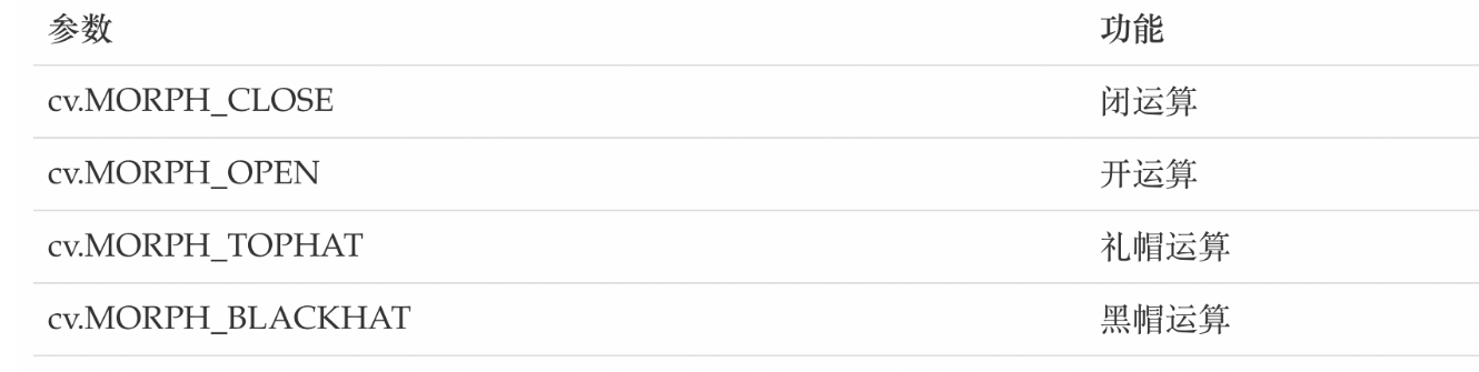
3. API

   cv.morphologyEx(img, op, kernel)
   

   Parameters:

   • img: image to process
   • op: processing method: if open operation is performed, it is set to CV MORPH_ Open, if closed operation is performed, it is set to CV MORPH_ CLOSE
   • kernel: core structure

4. Examples

   Implementation of opening and closing convolution using 10 * 10 kernel structure

   import numpy as np
   import cv2 as cv
   import matplotlib.pyplot as plt
   
   # 1 read image
   img1 = cv.imread("D:\Projects notes\opencv\image\letteropen.png")
   img2 = cv.imread("D:\Projects notes\opencv\image\letterclose.png")
   # 2 create core structure
   kernel = np.ones((10, 10), np.uint8)
   # 3 opening and closing operation of image
   cvopen = cv.morphologyEx(img1, cv.MORPH_OPEN, kernel)        # Open operation
   cvclose = cv.morphologyEx(img2, cv.MORPH_CLOSE, kernel)      # Closed operation
   # 4 image display
   fig, axes = plt.subplots(nrows=2, ncols=2, figsize=(10, 8), dpi=100)
   plt.rcParams['font.sans-serif'] = ['SimHei']    # Used to display Chinese normally
   axes[0, 0].imshow(img1)
   axes[0, 0].set_title("Original drawing")
   axes[0, 1].imshow(cvopen)
   axes[0, 1].set_title("Open operation result")
   axes[1, 0].imshow(img2)
   axes[1, 0].set_title("Original drawing")
   axes[1, 1].imshow(cvclose)
   axes[1, 1].set_tit
   le("Closed operation result")
   plt.show()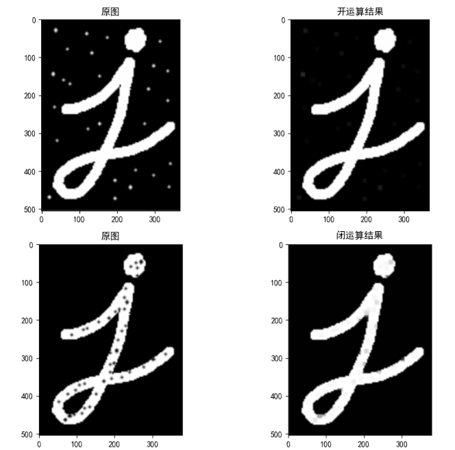
   

   

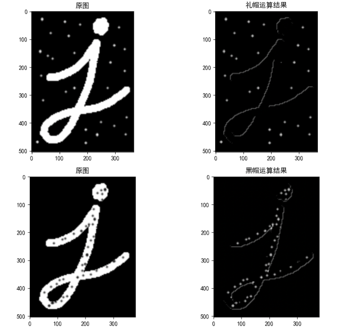
2.3 top hat and black hat

1. Top hat operation

   The difference between the original image and the result of "open operation" is calculated as follows:
   d s t = t o p h a t ( s r c , e l e m e n t ) = s r c − o p e n ( s r c , e l e m e n t ) dst = tophat(src, element) = src - open(src, element) dst=tophat(src,element)=src−open(src,element)
   Because the result of the open operation is to enlarge the crack or local low brightness area, the effect image obtained by subtracting the image after the open operation from the original image highlights the area brighter than the area around the outline of the original image, and this operation is related to the size of the selected core.

   The top hat operation is used to separate patches that are brighter than the adjacent ones. When an image has a large background and small objects are regular, the top hat operation can be used for background extraction.

2. Black hat operation

   Is the difference between the result image of "closed operation" and the original image. The mathematical expression is:
   d s t = b l a c k h a t ( s r c , e l e m e n t ) = c l o s e ( s r c , e l e m e n t ) − s r c dst = blackhat(src, element) = close(src, element) - src dst=blackhat(src,element)=close(src,element)−src
   The effect image after black hat operation highlights the darker area than the area around the outline of the original image, and this operation core is related to the size of the selected core.

   Black hat operation is used to separate patches darker than adjacent points.

3. API

   cv.morphologyEx(img, op, kernel)
   

   Parameters:

   • img: image to process

   • op: processing method:

     

   • kernel: core structure

   4. Examples

   import numpy as np
   import cv2 as cv
   import matplotlib.pyplot as plt
   
   # 1 read image
   img1 = cv.imread("D:\Projects notes\opencv\image\letteropen.png")
   img2 = cv.imread("D:\Projects notes\opencv\image\letterclose.png")
   # 2 create core structure
   kernel = np.ones((10, 10), np.uint8)
   # Black hat and black hat
   cvOpen = cv.morphologyEx(img1, cv.MORPH_TOPHAT, kernel)        # Top hat operation
   cvClose = cv.morphologyEx(img2, cv.MORPH_BLACKHAT, kernel)     # Black hat operation
   # 4 image display
   fig, axes = plt.subplots(nrows=2, ncols=2, figsize=(10, 8), dpi=100)
   plt.rcParams['font.sans-serif'] = ['SimHei']    # Used to display Chinese normally
   axes[0, 0].imshow(img1)
   axes[0, 0].set_title("Original drawing")
   axes[0, 1].imshow(cvOpen)
   axes[0, 1].set_title("Top hat calculation result")
   axes[1, 0].imshow(img2)
   axes[1, 0].set_title("Original drawing")
   axes[1, 1].imshow(cvClose)
   axes[1, 1].set_title("Black hat operation result")
   plt.show()
   

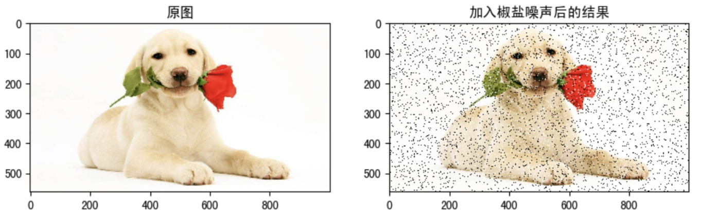
3 image smoothing

Because the process of image acquisition, processing and transmission will inevitably be polluted by noise, which hinders people's understanding, analysis and processing of images. Common image noises include Gaussian noise, salt and pepper noise and so on.

1 image noise

1.1 salt and pepper noise

Salt and pepper noise, also known as impulse noise, is a kind of noise often seen in images. It is a kind of random white or black spots. It may be that there are black pixels in bright areas or white pixels in dark areas (or both). Salt and pepper noise may be caused by sudden strong interference of image signal, analog-to-digital converter or bit transmission error. For example, a failed sensor causes the pixel value to be the minimum value, and a saturated sensor causes the pixel value to be the maximum value.

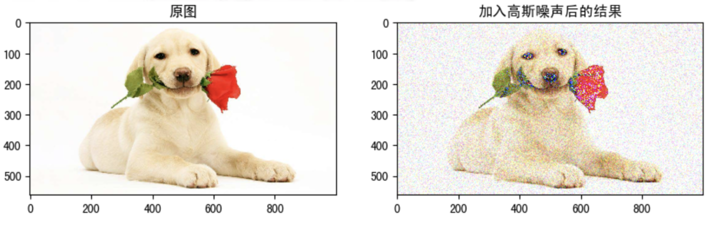
1.2 Gaussian noise

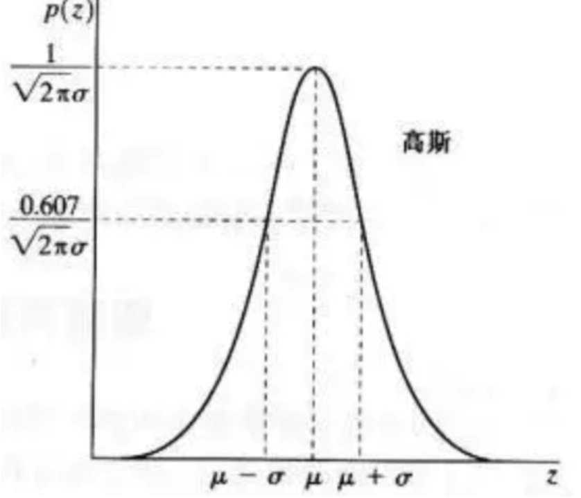
Gaussian noise is a kind of noise whose noise density function obeys Gaussian distribution. Due to the mathematical ease of Gaussian noise in space and frequency domain, this noise (also known as normal noise) model is often used in practice. The probability density function of Gaussian random variable z is given by the following formula:
p ( z ) = 1 2 π σ e − ( z − μ ) 2 2 σ 2 p(z) = \frac{1}{\sqrt{2\pi}\sigma}e^\frac{-(z-\mu)^2}{2\sigma^2} p(z)=2π ​σ1​e2σ2−(z−μ)2​
Where z represents the gray value, μ \mu μ Represents the average or expected value of z, σ \sigma σ Represents the standard deviation of z. Square of standard deviation σ 2 \sigma^2 σ 2 is called the variance of z. The curve of Gaussian function is shown in the figure:

2 Introduction to image smoothing

From the perspective of signal processing, image smoothing is to remove the high-frequency information and retain the low-frequency information. Therefore, we can implement low-pass filtering on the image. Low pass filtering can remove the noise in the image and smooth the image.

According to different filters, they can be divided into mean filter, Gaussian filter, median filter and bilateral filter.

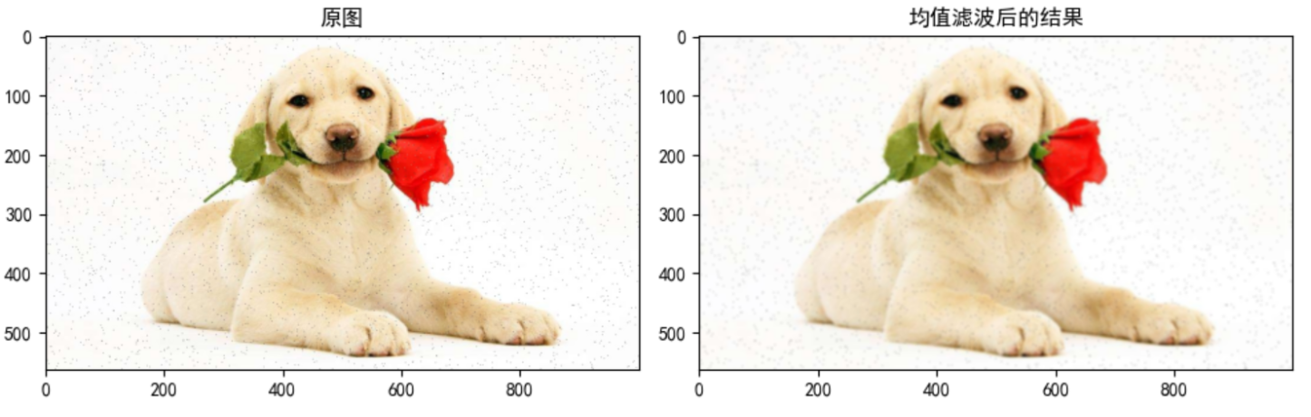
2.1 mean filtering

The mean filtering template is used to filter the image noise. order S x y S_{xy} Sxy ＾ represents the coordinate group of the rectangular sub image window with the center at point (x, y) and the size of mxn. The mean filter can be expressed as:
f ^ ( x , y ) = 1 m n ∑ ( s , t ) ∈ S x y g ( s , t ) \widehat{f}(x,y)=\frac{1}{mn}\sum_{(s,t)\in S_{xy}}{g(s,t)} f ​(x,y)=mn1​(s,t)∈Sxy​∑​g(s,t)
It is completed by a normalized convolution frame. It replaces the central element with the average value of all pixels in the coverage area of the convolution frame.

For example, the 3x3 standardized average filter is as follows:
K = 1 9 [ 1 1 1 1 1 1 1 1 1 ] (3) K=\frac{1}{9}\left[ \begin{matrix} 1 & 1 & 1 \\ 1 & 1 & 1 \\ 1 & 1 & 1 \end{matrix} \right] \tag{3} K=91​⎣⎡​111​111​111​⎦⎤​(3)
The advantage of mean filtering is that the algorithm is simple and the calculation speed is fast. The disadvantage is that many details are removed while denoising, which makes the image blurred.

API:

cv.blur(src, ksize, anchor, borderType)

Parameters:

• src: input image
• ksize: size of convolution kernel
• anchor: the default value (- 1, - 1) indicates the core center
• borderYType: boundary type

Example:

from matplotlib import pyplot as plt
import cv2 as cv
import numpy as np

# 1 image reading
img = cv.imread("D:\Projects notes\opencv\image\dogsp.jpeg")
# 2-means filtering
blur = cv.blur(img, (5, 5))
# 3 image display
fig, axes = plt.subplots(nrows=1, ncols=2, figsize=(10, 8), dpi=100)
plt.rcParams['font.sans-serif'] = ['SimHei']    # Used to display Chinese normally
axes[0].imshow(img[:, :, ::-1])
axes[0].set_title("Original drawing")
axes[1].imshow(blur[:, :, ::-1])
axes[1].set_title("Structure after corrosion")
plt.show()

2.2 Gaussian filtering

Two dimensional Gaussian filter is the basis of constructing Gaussian filter, and its probability distribution function is as follows:
G ( x , y ) = 1 2 π σ 2 e x p { − x 2 + y 2 2 σ 2 } (6) G(x,y) = \frac{1}{2\pi \sigma^2}exp\begin{Bmatrix} -\frac{x^2+y^2}{2\sigma^2} \end{Bmatrix} \tag{6} G(x,y)=2πσ21​exp{−2σ2x2+y2​​}(6)
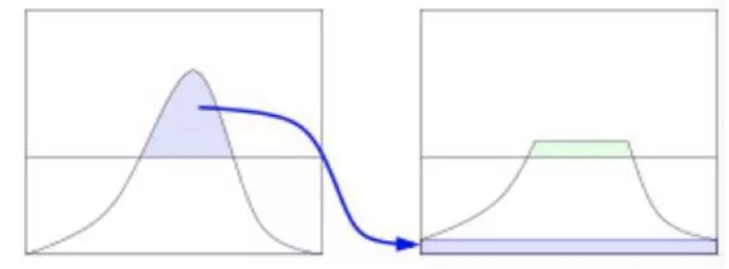
The distribution of G (x, y) is a prominent hat shape here σ \sigma σ It can be regarded as two values. One is the standard deviation in the x direction σ x \sigma_x σ x, the other is the standard deviation in the y direction σ y \sigma_y σy​.

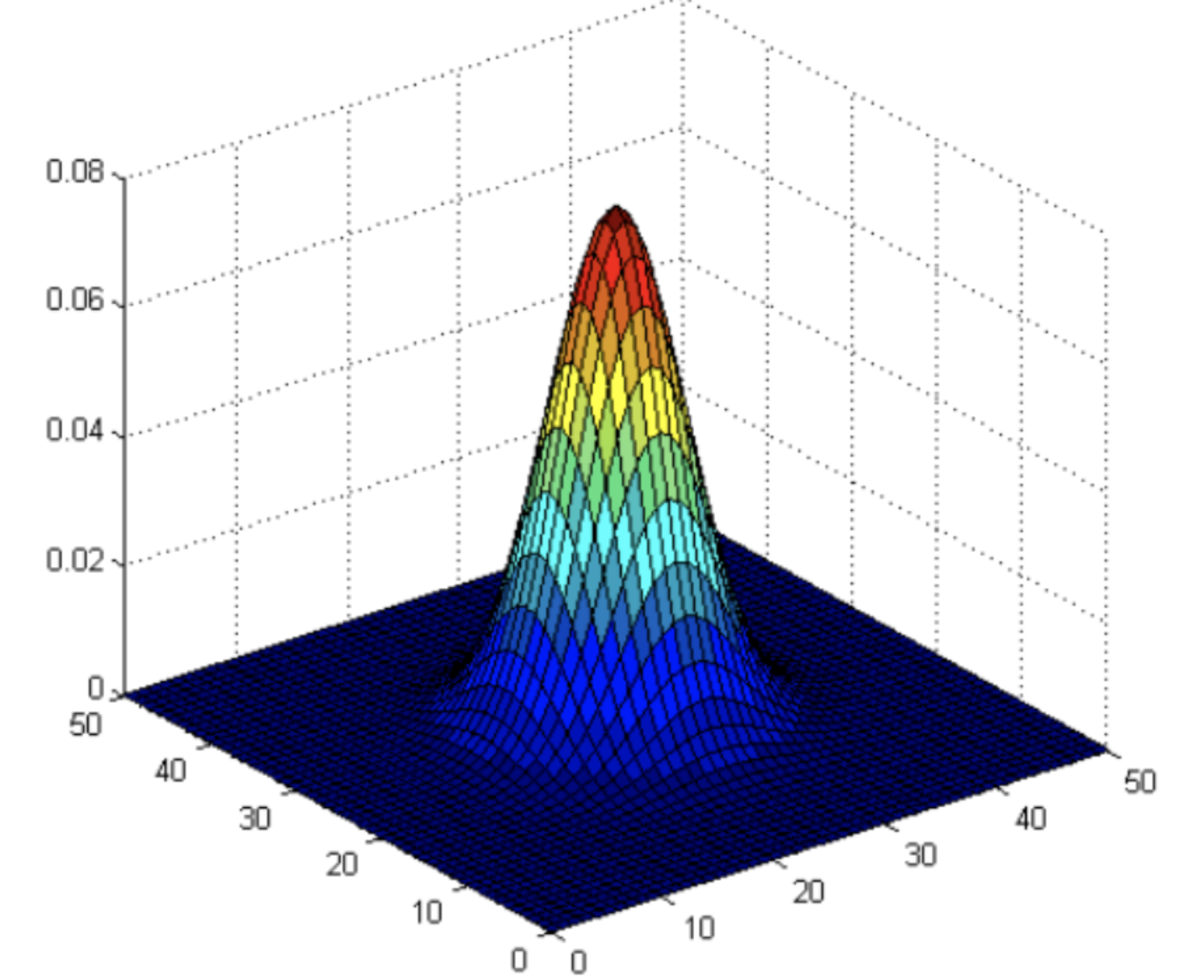
When σ x \sigma_x σ x ， and σ y \sigma_y σ The larger the value of y, the whole shape tends to be flat; When σ x \sigma_x σ x ， and σ y \sigma_y σ The smaller the value of y ， the more prominent the whole shape is

Normal distribution is a bell curve. The closer it is to the center, the greater the value. The farther it is away from the center, the smaller the value. When calculating the smoothing result, you only need to take the "center point" as the origin and assign weights to other points according to their positions on the normal curve to obtain a weighted average.

Gaussian smoothing is very effective in removing Gaussian noise from images.

Gaussian smoothing process:

• Firstly, the weight matrix is determined

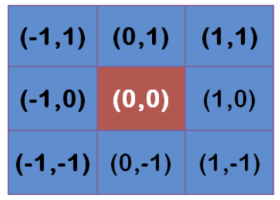
Assuming that the coordinates of the center point are (0, 0), the coordinates of the 8 closest points are as follows:

Further points, and so on.

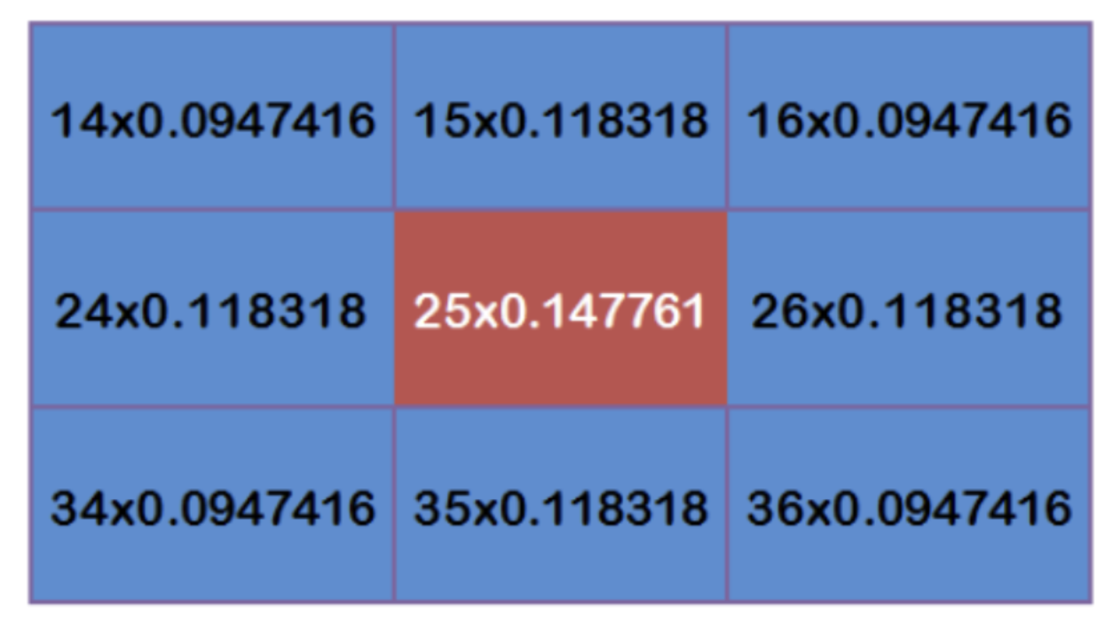
In order to calculate the weight matrix, you need to set σ \sigma σ Value of. assume σ = 1.5 \sigma=1.5 σ= 1.5, the weight matrix with fuzzy radius of 1 is as follows:

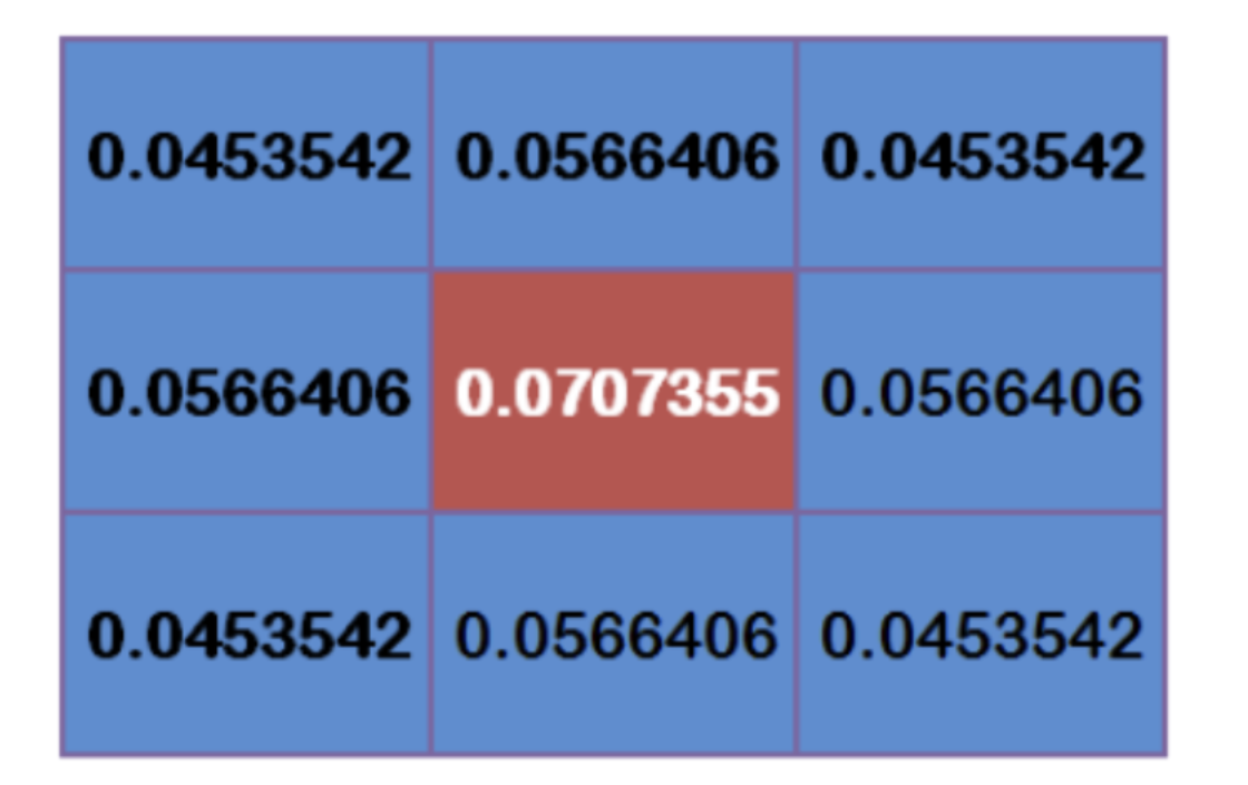
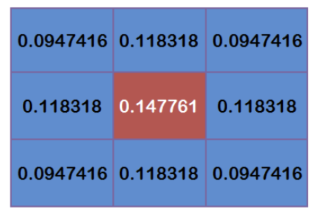
The total weight of these nine points is equal to 0.4787147. If only the weighted average of these nine points is calculated, the sum of their weights must be equal to 1. Therefore, the above nine values must be divided by 0.4787147 respectively to obtain the final weight matrix.

• Calculate Gaussian blur

With the weight matrix, the value of Gaussian blur can be calculated.

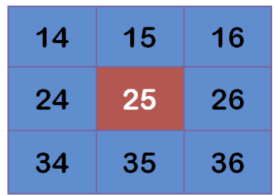
Assuming that there are 9 pixels, the gray value (0-255) is as follows:

Multiply each point by the corresponding weight value:

Get:

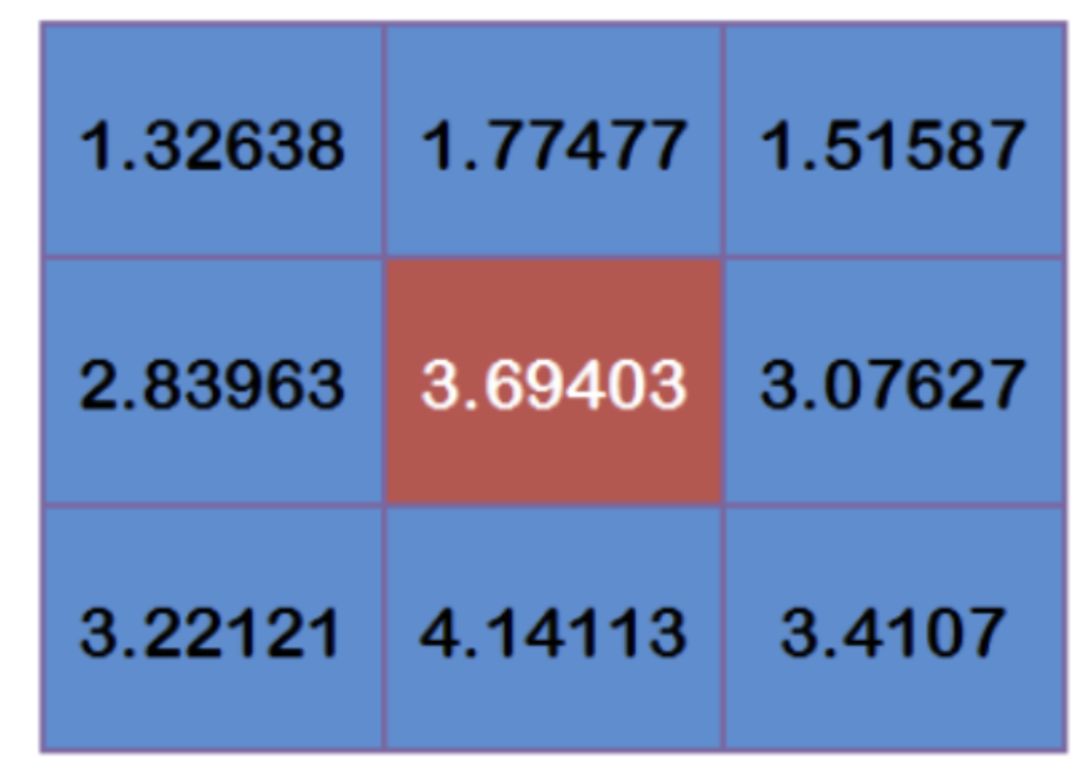
Add up these nine values to get the Gaussian blur value of the center point.

Repeat this process for all points to get the Gaussian blurred image. If the original image is a color image, Gaussian smoothing can be performed on the three RGB channels respectively.

API:

cv2.GaussianBlur(src, ksize, sigmaX, sigmaY, borderType)

Parameters:

• src: input image
• ksize: the size of Gaussian convolution kernel. Note: the width and height of convolution kernel should be odd and can be different
• Sigma X: standard deviation in horizontal direction
• sigmaY: the standard deviation in the vertical direction. The default value is 0, which means it is the same as sigmaX
• borderType: fill boundary type

Example:

from matplotlib import pyplot as plt
import cv2 as cv
import numpy as np

# 1 image reading
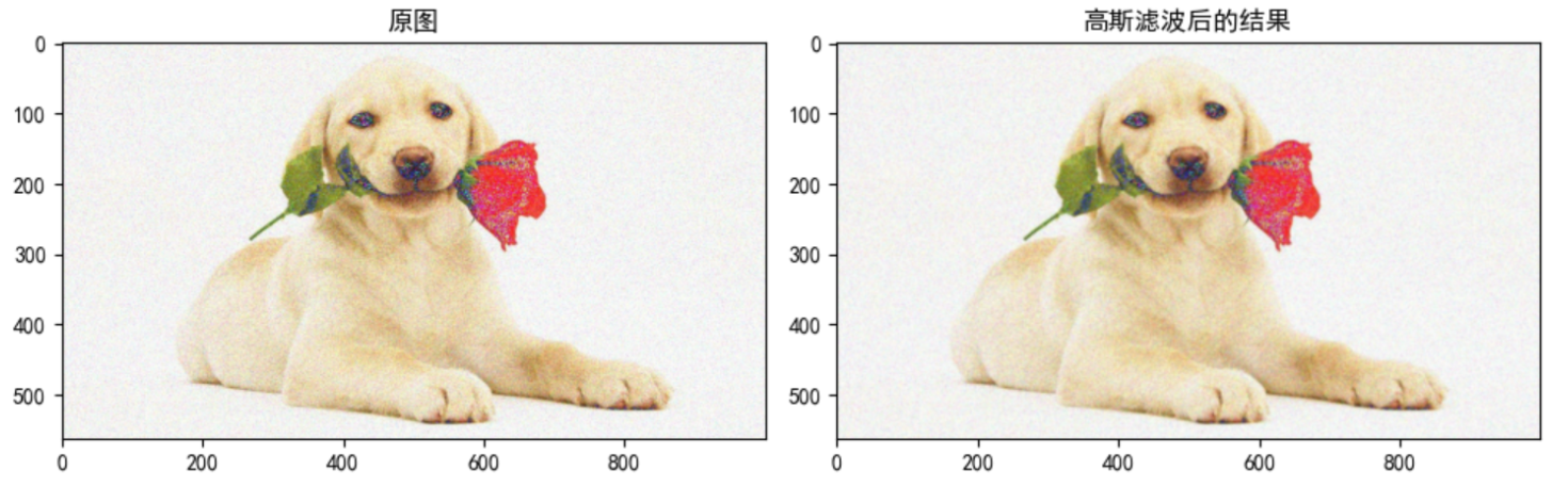
img = cv.imread("D:\Projects notes\opencv\image\dogGauss.jpeg")
# 2 Gaussian filtering
blur = cv.GaussianBlur(img, (3, 3), 1)
# 3 image display
fig, axes = plt.subplots(nrows=1, ncols=2, figsize=(10, 8), dpi=100)
plt.rcParams['font.sans-serif'] = ['SimHei']    # Used to display Chinese normally
axes[0].imshow(img[:, :, ::-1])
axes[0].set_title("Original drawing")
axes[1].imshow(blur[:, :, ::-1])
axes[1].set_title("Results after Gaussian filtering")
plt.show()

2.3 median filtering

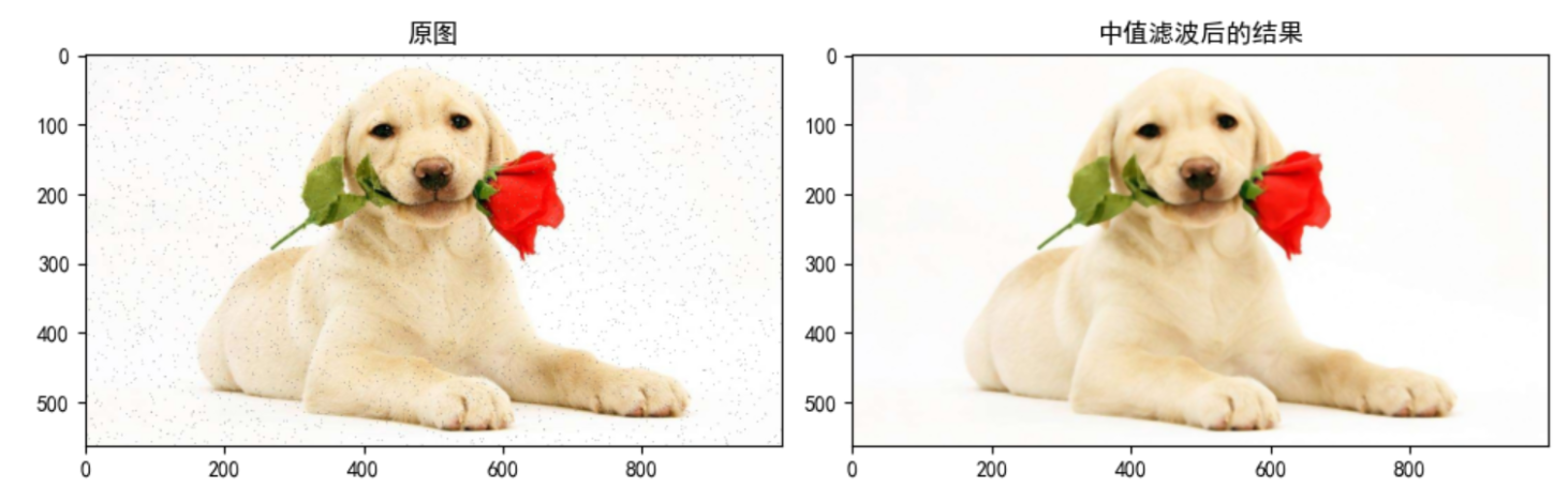
Median filtering is a typical nonlinear filtering technology. The basic idea is to replace the gray value of the pixel with the median of the gray value in the neighborhood of the pixel.

Median filtering is particularly useful for salt and pepper noise because it does not depend on the values in the neighborhood that are very different from the typical values.

API:

cv.medianBlur(src, ksize)

Parameters:

• src: input image
• ksize: size of convolution kernel

Example:

from matplotlib import pyplot as plt
import cv2 as cv
import numpy as np

# 1 image reading
img = cv.imread("D:\Projects notes\opencv\image\dogsp.jpeg")
# 2 Gaussian filtering
blur = cv.medianBlur(img, 5)
# Display image 3
fig, axes = plt.subplots(nrows=1, ncols=2, figsize=(10, 8), dpi=100)
plt.rcParams['font.sans-serif'] = ['SimHei']    # Used to display Chinese normally
axes[0].imshow(img[:, :, ::-1])
axes[0].set_title("Original drawing")
axes[1].imshow(blur[:, :, ::-1])
axes[1].set_title("Results after median filtering")
plt.show()

3 histogram

3.1 gray histogram

1. principle

Histogram is a method of data statistics, and organizes the statistical values into a series of bin defined by the implementation. Among them, bin is a concept often used in histogram, which can be translated as "straight bar" or "group distance". Its value is the feature statistics calculated from the data, which can be such as gradient, direction, color or any other feature.

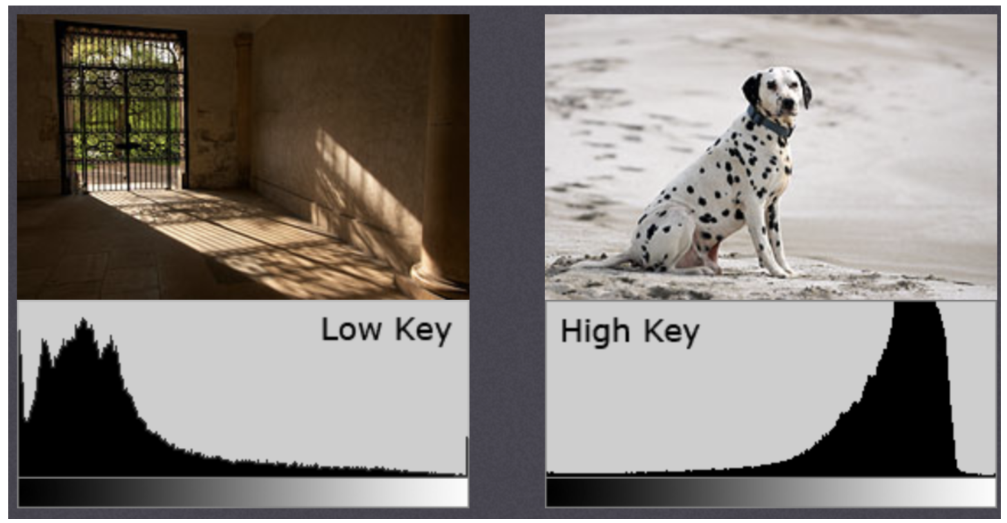
Image histogram is a histogram used to represent the brightness distribution in digital image. It plots the number of pixels of each brightness value in the image. In this histogram, the left side of the abscissa is a darker area and the right side is a brighter area. Therefore, the data in the histogram of a darker image is mostly concentrated in the left and middle parts, while the image with bright overall and only a small amount of shadow is the opposite.

Note: the histogram is drawn according to the gray image, not the color image.

Assuming that there is information of an image (gray value 0-255), the range of known numbers contains 256 values, so this range can be divided into sub regions (i.e. bins) according to a certain law. For example:
[ 0 , 255 ] = [ 0 , 15 ] ∪ [ 16 , 30 ] ⋯ ∪ [ 240 , 255 ] [0, 255]=[0,15]\cup[16,30]\cdots\cup[240,255] [0,255]=[0,15]∪[16,30]⋯∪[240,255]
Then count the number of pixels of each bin(i). The following figure can be obtained (where x-axis represents bin and y-axis represents the number of pixels in each bin):

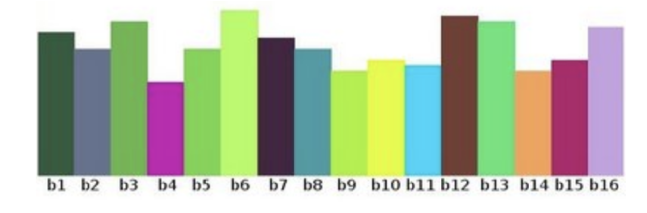
Some terms and details in the histogram:

• Dims: the number of features to be counted. In the above example, dims=1, because only the gray value is counted
• Bins: the number of sub segments of each feature space, which can be translated as "straight bar" or "group distance". In the above example, bins=16
• Range: the value range of the feature to be counted. In the above example, range = [0255]

Significance of histogram:

• Histogram is an image representation of pixel intensity distribution in an image
• It counts the number of pixels of each intensity value
• The histograms of different images may be the same

1. Calculation and drawing of histogram

Use the method in opencv to count the histogram and draw it with matplotlib

API:

cv2.calcHist(images, channels, mask, histSize, ranges[, hist[, accumulate]])

Parameters:

• images: the original image, which should be enclosed in brackets [] when passing in a function, for example: [img]
• Channels: if the input image is a grayscale image, its value is [0]; If it is a color image, the parameters passed in can be [0], [1], [2]. They use channels B, G and R respectively
• Mask: mask image. To count the histogram of the whole image, set it to None. But if you want to count the histogram of a part of the image, you need to make a mask image and use it (there are examples later)
• histSize: the number of bin should also be enclosed in brackets, for example: [256]
• ranges: range of pixel values, usually [0, 256]

Example:

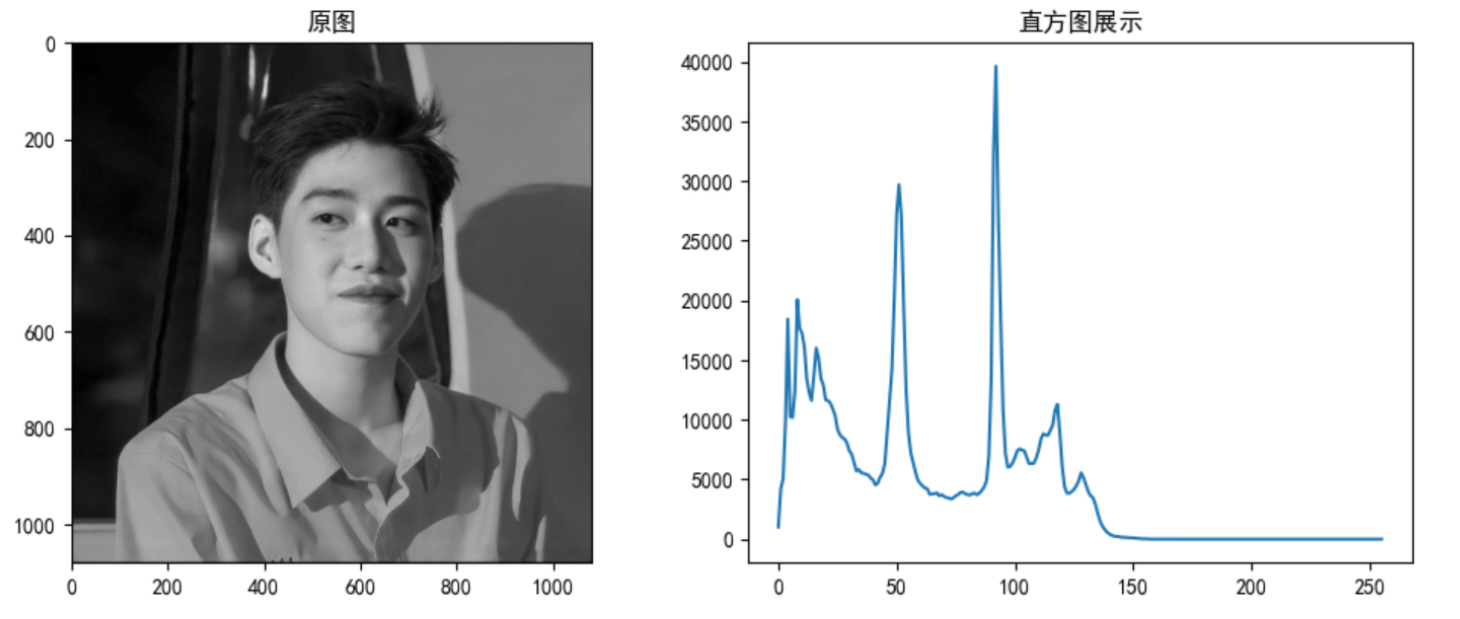
As shown in the figure below, draw the corresponding histogram

import numpy as np
import cv2 as cv
from matplotlib import pyplot as plt

# 1. Read directly in the form of gray image
img = cv.imread("D:\Projects notes\opencv\image\_20201226153617.jpg", 0)
# 2 Statistical grayscale image
histr = cv.calcHist([img], [0], None, [256], [0, 256])
# 3 draw histogram
fig, axes = plt.subplots(nrows=1, ncols=2, figsize=(10, 8), dpi=100)
plt.rcParams['font.sans-serif'] = ['SimHei']    # Used to display Chinese normally
axes[0].imshow(img, cmap=plt.cm.gray)
axes[0].set_title("Original drawing")
axes[1].plot(histr)
axes[1].set_title("Results after median filtering")
plt.show()

1. Application of mask

Mask uses the selected image, figure or object to block the image to be processed to control the area of graphic processing.

In digital image processing, we usually use two-dimensional matrix array for mask. The mask is a binary image composed of 0 and 1. The mask image is used to mask the image to be processed, in which the 1 value area is processed, and the 0 value area is shielded and will not be processed.

The main uses of the mask are:

• Extracting the region of interest: use the pre made mask of the region of interest and the image to be processed to obtain the image of the region of interest. The image value in the region of interest remains unchanged, while the image value outside the region of interest is 0
• Shielding function: mask some areas on the image so that they do not participate in the processing or calculation of processing parameters, or only process or count the shielding area.
• Structural feature extraction: detect and extract the structural features similar to the mask in the image by similarity variable or image matching method.
• Special shape image making

Masks are widely used in remote sensing image processing. When extracting roads, rivers or houses, a mask matrix is used to filter the pixels of the image, and then the features or signs we need are highlighted.

Use cv Calchist() to find the histogram of the complete image. If you want to find the histogram of some areas of the image, just create a white mask image on the area where you want to find the histogram, otherwise create black, and then transfer it as a mask mask.

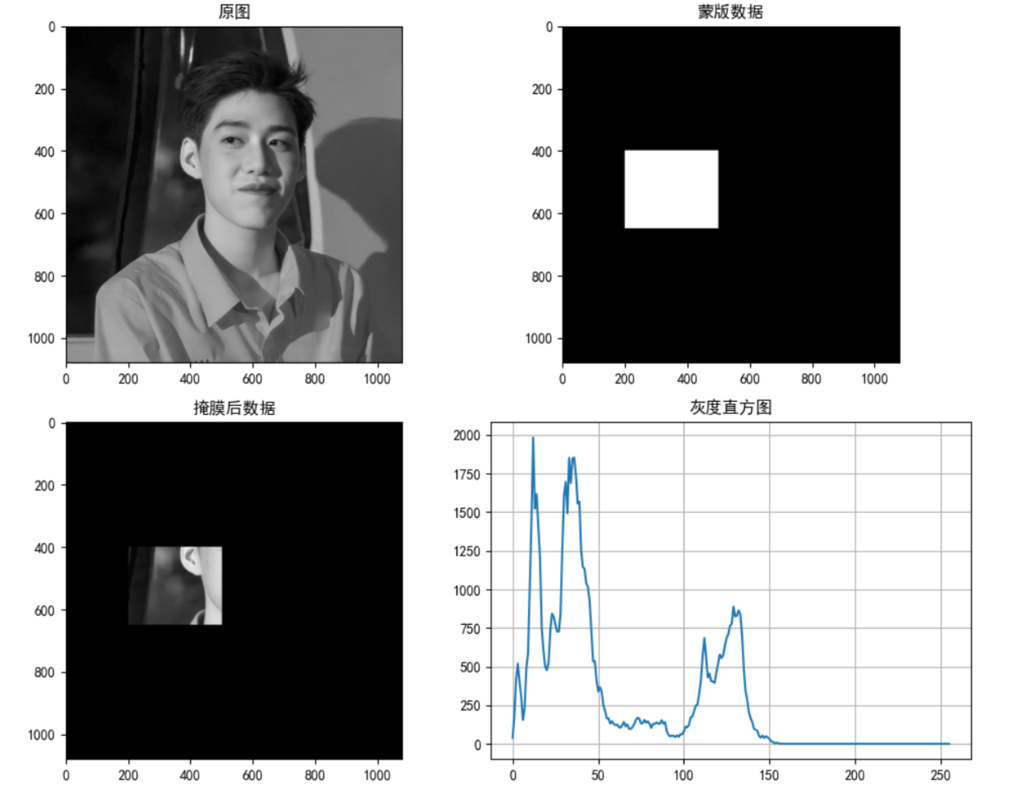
Example:

import numpy as np
import cv2 as cv
from matplotlib import pyplot as plt

# 1. Read directly in the form of gray image
img = cv.imread("D:\Projects notes\opencv\image\_20201226153617.jpg", 0)
# 2 create mask
mask = np.zeros(img.shape[:2], np.uint8)
mask[400:650, 200:500] = 255
# 3 mask
masked_img = cv.bitwise_and(img, img, mask=mask)
# 4. Count the gray image of the image after the mask
mask_histr = cv.calcHist([img], [0], mask, [256], [1, 256])
# 5 image display
fig, axes = plt.subplots(nrows=2, ncols=2, figsize=(10, 8), dpi=100)
plt.rcParams['font.sans-serif'] = ['SimHei']    # Used to display Chinese normally
axes[0, 0].imshow(img, cmap=plt.cm.gray)
axes[0, 0].set_title("Original drawing")
axes[0, 1].imshow(mask, cmap=plt.cm.gray)
axes[0, 1].set_title("Mask data")
axes[1, 0].imshow(masked_img, cmap=plt.cm.gray)
axes[1, 0].set_title("Post mask data")
axes[1, 1].plot(mask_histr)
axes[1, 1].grid()
axes[1, 1].set_title("Gray histogram")
plt.show()

3.2 histogram equalization

1. Principle and Application

Imagine if the pixel values of most pixels in an image are concentrated in a small gray value range? If an image is bright as a whole, the number of pixel values should be high. Therefore, its histogram should be stretched horizontally (as shown in the figure below), which can expand the distribution range of image pixel values and improve the image contrast. This is what histogram equalization should do.

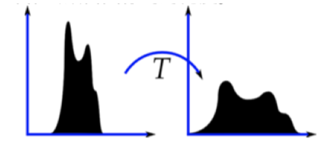
"Histogram equalization" is to change the gray histogram of the original image from a relatively concentrated gray range to a distribution in a wider gray range. Histogram equalization is to stretch the image nonlinearly and redistribute the image pixel values to make the number of pixels in a certain gray range roughly the same.

This method improves the overall contrast of the image, especially when the pixel value distribution of useful data is relatively close, it is widely used in X-ray images, which can improve the display of skeleton structure. In addition, it can better highlight details in overexposed or underexposed images.

When using opencv for histogram statistics, the following are used:

API:

dst = cv.equalizeHist(img)

Parameters:

• img: grayscale image

return:

• dst: results after equalization

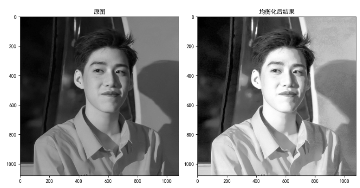
Example:

import numpy as np
import cv2 as cv
from matplotlib import pyplot as plt

# 1. Read directly in the form of gray image
img = cv.imread("D:\Projects notes\opencv\image\_20201226153617.jpg", 0)
# 2. Equalization treatment
dst = cv.equalizeHist(img)
# 3. Result display
fig, axes = plt.subplots(nrows=1, ncols=2, figsize=(10, 8), dpi=100)
plt.rcParams['font.sans-serif'] = ['SimHei']    # Used to display Chinese normally
axes[0].imshow(img, cmap=plt.cm.gray)
axes[0].set_title("Original drawing")
axes[1].imshow(dst, cmap=plt.cm.gray)
axes[1].set_title("Results after equalization")
plt.show()

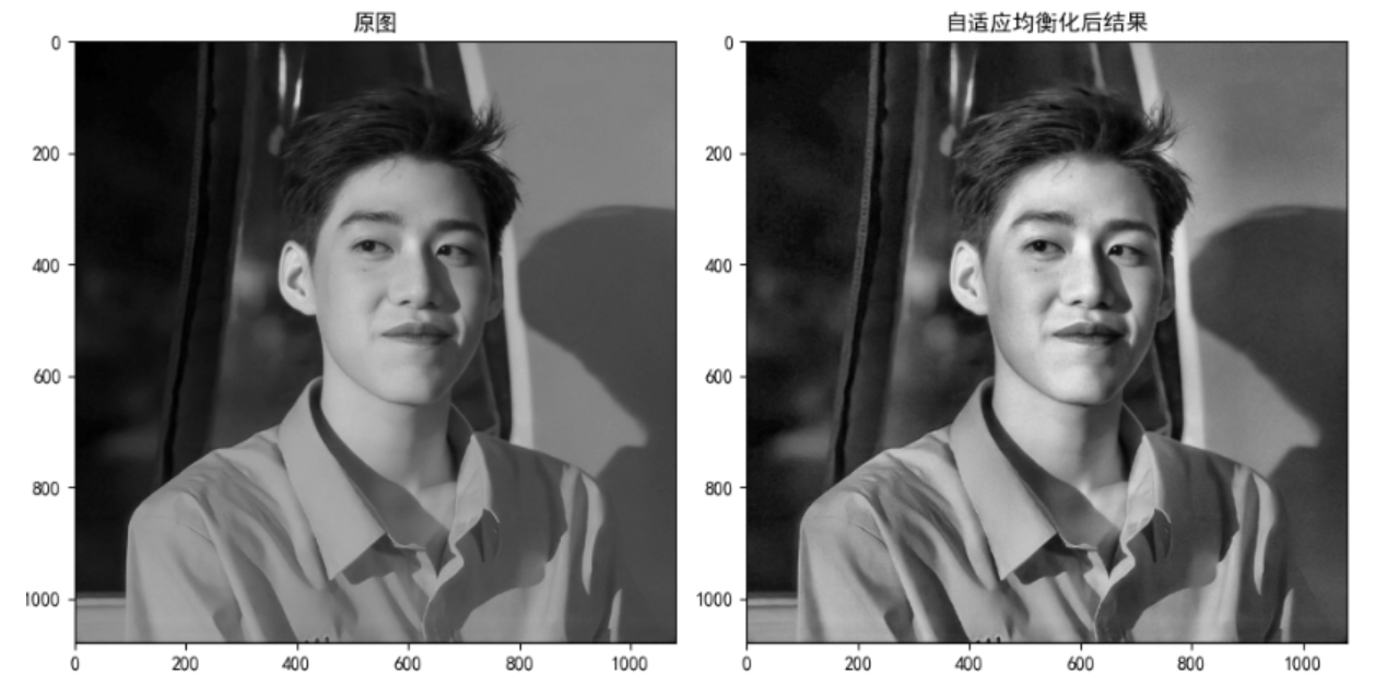
3.3 adaptive histogram equalization

In the above histogram equalization, we consider the global contrast of the image. As shown in the figure below, comparing the images of the statues in the next two pictures, a lot of information is lost because they are too bright.

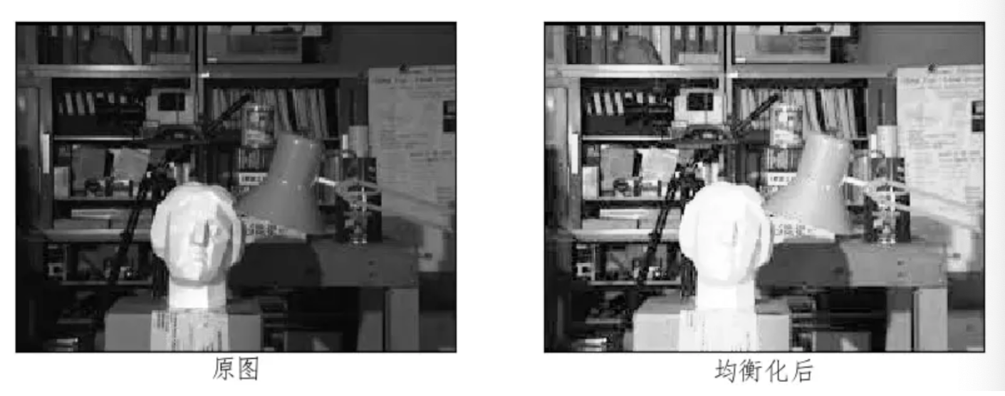
In order to solve this problem, adaptive histogram equalization is needed. At this time, the whole image will be divided into many small blocks, which are called "tiles" (the default size of tiles in opencv is 8 * 8), and then each small block will be and retrograde histogram equalized respectively. Therefore, in each region, the histogram will be concentrated in a small region). If the noise is, the noise will be amplified. To avoid this, use contrast limits. For each small block, if the bin in the histogram exceeds the upper limit of contrast, the pixels in it will be evenly dispersed into other bins, and then histogram equalization will be carried out.

Finally, in order to remove the boundary between each block, bilinear interpolation is used to splice each block.

API:

cv.createCLAHE(clipLimit, tileGridSize)

Parameters:

• clipLimit: contrast limit. The default value is 40
• tileGridSize: block size. The default value is 8 * 8

Example:

import numpy as np
import cv2 as cv
from matplotlib import pyplot as plt

# 1. Read directly in the form of gray image
img = cv.imread("D:\Projects notes\opencv\image\_20201226153617.jpg", 0)
# 2 create an adaptive equalization object and apply it to the image
clahe = cv.createCLAHE(clipLimit=2.0, tileGridSize=(8, 8))
cl1 = clahe.apply(img)
# 3 image display
fig, axes = plt.subplots(nrows=1, ncols=2, figsize=(10, 8), dpi=100)
plt.rcParams['font.sans-serif'] = ['SimHei']    # Used to display Chinese normally
axes[0].imshow(img, cmap=plt.cm.gray)
axes[0].set_title("Original drawing")
axes[1].imshow(cl1, cmap=plt.cm.gray)
axes[1].set_title("Results after adaptive equalization")
plt.show()

Summary:

1. Gray histogram:

• Histogram is an image expression of pixel intensity distribution in an image.
• It counts the number of pixels of each intensity value
• The histograms of different images may be the same

cv2.calcHist(images, channels, mask, histSize, ranges[, hist[, accumulate]])

1. Mask

Create a mask and pass it through the mask to obtain the histogram of the region of interest

1. A method of image contrast equalization based on histogram

​ cv.equalizeHist(): the input is a grayscale image and the output is a histogram equalization image

1. Adaptive histogram equalization

The whole image is divided into many small blocks, then each small block is histogram equalized, and finally spliced

     clahe = cv.createCLAHE(clipLimit, tileGridsize)