OpenCV image processing
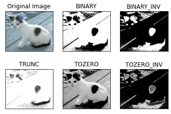
1. Image threshold
ret, dst = cv2.threshold(src, thresh, maxval, type)
- src: input image, only single channel image can be input, usually gray image
- dst: output diagram
- thresh: threshold
- maxval: the value assigned when the pixel value exceeds the threshold (or is less than the threshold, depending on the type)
- Type: the type of binarization operation, including the following five types:
- cv2.THRESH_BINARY: maxval (maximum value) is taken for the part exceeding the threshold, otherwise 0 is taken
- cv2.THRESH_BINARY_INV : THRESH_ Inversion of binary
- cv2.THRESH_TRUNC: the part greater than the threshold value is set as the threshold value, otherwise it remains unchanged
- cv2.THRESH_TOZERO: the part greater than the threshold does not change, otherwise it is set to 0
- cv2.THRESH_TOZERO_INV : THRESH_ Inversion of tozero
import cv2
import matplotlib.pyplot as plt

img=cv2.imread('../image/cat.jpg')
img_gray = cv2.cvtColor(img,cv2.COLOR_BGR2GRAY)
ret, thresh1 = cv2.threshold(img_gray, 127, 255, cv2.THRESH_BINARY)     # maxval (maximum value) is taken for the part exceeding the threshold value, otherwise 0 is taken
ret, thresh2 = cv2.threshold(img_gray, 127, 255, cv2.THRESH_BINARY_INV) # THRESH_ Inversion of binary
ret, thresh3 = cv2.threshold(img_gray, 127, 255, cv2.THRESH_TRUNC)      # The part greater than the threshold is set as the threshold, otherwise it remains unchanged
ret, thresh4 = cv2.threshold(img_gray, 127, 255, cv2.THRESH_TOZERO)     # The part greater than the threshold does not change, otherwise it is set to 0
ret, thresh5 = cv2.threshold(img_gray, 127, 255, cv2.THRESH_TOZERO_INV) # THRESH_ Inversion of tozero

titles = ['Original Image', 'BINARY', 'BINARY_INV', 'TRUNC', 'TOZERO', 'TOZERO_INV']
images = [img, thresh1, thresh2, thresh3, thresh4, thresh5]

for i in range(6):
    plt.subplot(2, 3, i + 1), plt.imshow(images[i], 'gray')
    plt.title(titles[i])
    plt.xticks([]), plt.yticks([])
plt.show()
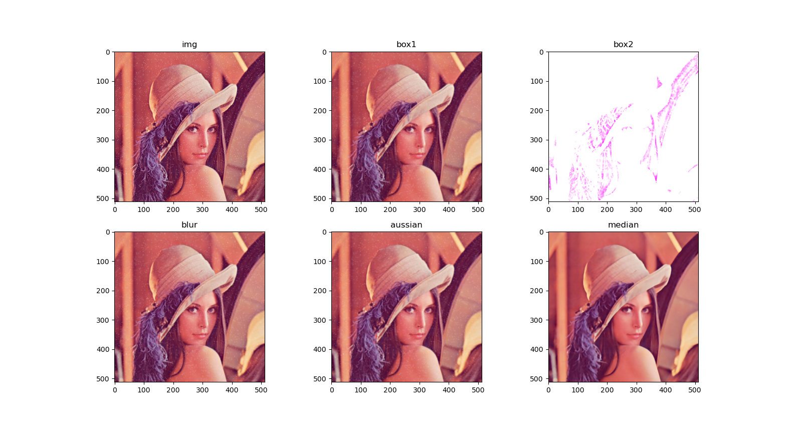
2. Image smoothing
import cv2
import matplotlib.pyplot as plt
import numpy as np

img = cv2.imread('../image/lenaNoise.png')[:,:,::-1] #cv2 displays bgr and plt displays rgb
# Mean filtering
# Simple average convolution operation
blur = cv2.blur(img, (3, 3))

# box filter
# Basically the same as the mean, normalization can be selected
box1 = cv2.boxFilter(img,-1,(3,3), normalize=True)

# box filter
# Basically the same as the mean value, normalization can be selected, which is easy to cross the boundary
box2 = cv2.boxFilter(img,-1,(3,3), normalize=False)

# Gaussian filtering
# The value in the convolution kernel of Gaussian blur satisfies the Gaussian distribution, which is equivalent to paying more attention to the middle
aussian = cv2.GaussianBlur(img, (5, 5), 1)

# median filtering
# Equivalent to replacing with median
median = cv2.medianBlur(img, 5)  # median filtering

# Show all
plt.subplot(231),plt.imshow(img,"gray"),plt.title("img")
plt.subplot(232),plt.imshow(box1),plt.title("box1")
plt.subplot(233),plt.imshow(box2),plt.title("box2")
plt.subplot(234),plt.imshow(blur),plt.title("blur")
plt.subplot(235),plt.imshow(aussian),plt.title("aussian")
plt.subplot(236),plt.imshow(median),plt.title("median")
plt.show()
3. Morphological operation
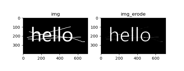
3.1 corrosion
Corrosion is very similar to expansion. It also convolutes the original image and arbitrarily shaped cores. The difference is that during the expansion operation, the kernel is crossed over the image, and the minimum pixel value covered by the kernel is extracted to replace the pixel at the anchor position. This operation will expand the "dark area" in the image.
import cv2
import numpy as np
import matplotlib.pyplot as plt

img = cv2.imread('../image/wz.png')

kernel = np.ones((3,3),np.uint8)
img_erode = cv2.erode(img,kernel,iterations = 2) #corrosion

plt.subplot(121),plt.imshow(img,"gray"),plt.title("img")
plt.subplot(122),plt.imshow(img_erode,"gray"),plt.title("img_erode")
plt.show()
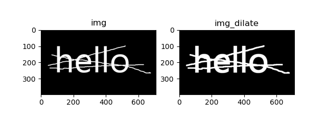
3.2 expansion
The expansion operation is to convolute the original graph and the kernel of any shape. There is a definable anchor point in the kernel, which is called the kernel center point. During the expansion operation, the kernel is crossed over the image, and the maximum pixel value covered by the kernel is extracted to replace the pixel at the anchor position. This operation will expand the "bright area" in the image.
import cv2
import numpy as np
import matplotlib.pyplot as plt

img = cv2.imread('../image/wz.png')

kernel = np.ones((3,3),np.uint8)
img_dilate = cv2.dilate(img,kernel,iterations = 2) #expand

plt.subplot(121),plt.imshow(img,"gray"),plt.title("img")
plt.subplot(122),plt.imshow(img_dilate,"gray"),plt.title("img_dilate")
plt.show()
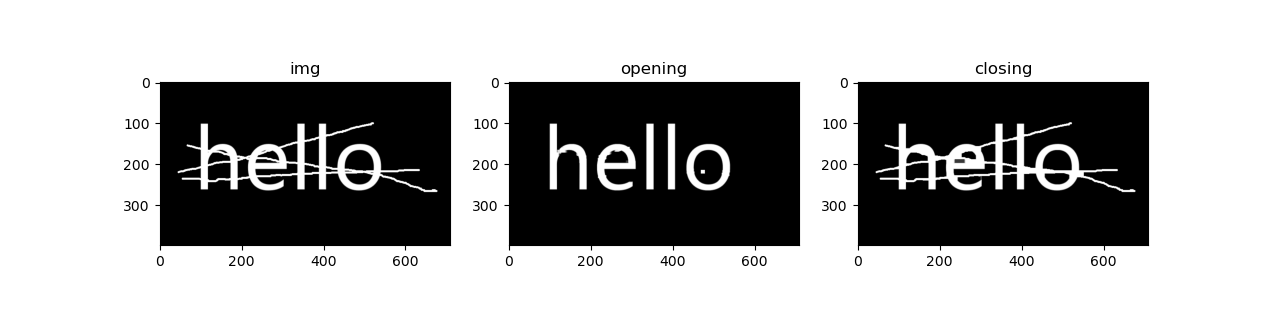
3.3 open and close operations
Similarities and differences between open operation and closed operation
import cv2
import numpy as np
import matplotlib.pyplot as plt

img = cv2.imread('../image/wz.png')

kernel = np.ones((5,5),np.uint8)
# On: first corrosion, then expansion
opening = cv2.morphologyEx(img, cv2.MORPH_OPEN, kernel)

# Closed: expand first and then corrode
closing = cv2.morphologyEx(img, cv2.MORPH_CLOSE, kernel)

plt.subplot(131),plt.imshow(img,"gray"),plt.title("img")
plt.subplot(132),plt.imshow(opening,"gray"),plt.title("opening")
plt.subplot(133),plt.imshow(closing,"gray"),plt.title("closing")
plt.show()
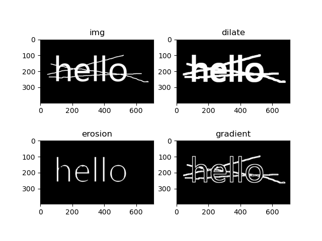
3.4 gradient operation
Gradient = expansion corrosion
import cv2
import numpy as np
import matplotlib.pyplot as plt

img = cv2.imread('../image/wz.png')

kernel = np.ones((5,5),np.uint8)
dilate = cv2.dilate(img,kernel,iterations = 2)
erosion = cv2.erode(img,kernel,iterations = 2)

gradient = cv2.morphologyEx(img, cv2.MORPH_GRADIENT, kernel)

plt.subplot(221),plt.imshow(img,"gray"),plt.title("img")
plt.subplot(222),plt.imshow(dilate,"gray"),plt.title("dilate")
plt.subplot(223),plt.imshow(erosion,"gray"),plt.title("erosion")
plt.subplot(224),plt.imshow(gradient,"gray"),plt.title("gradient")
plt.show()
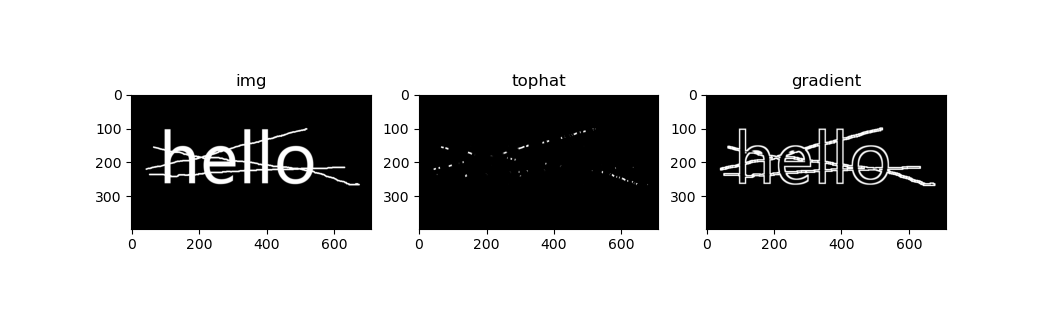
3.5 top hat and black hat
-
Top hat = original input - open operation result
-
Black hat = closed operation - original input
import cv2
import numpy as np
import matplotlib.pyplot as plt

img = cv2.imread('../image/wz.png')

kernel = np.ones((5,5),np.uint8)
tophat = cv2.morphologyEx(img, cv2.MORPH_TOPHAT, kernel) #formal hat

gradient = cv2.morphologyEx(img, cv2.MORPH_GRADIENT, kernel) #Black hat

plt.subplot(131),plt.imshow(img,"gray"),plt.title("img")
plt.subplot(132),plt.imshow(tophat,"gray"),plt.title("tophat")
plt.subplot(133),plt.imshow(gradient,"gray"),plt.title("gradient")
3.6 getStructuringElement()
Morphological operations are often used in image processing, in which structural elements must be obtained first. Including the size and shape of structural elements. cv2.getStructuringElement() returns a structure element of a specific size and shape for morphological operations.
Using Numpy to build structured elements is square. But sometimes we need to build an oval / circular core. In order to achieve this requirement, the OpenCV function CV2 is provided getStructuringElement(). You just need to tell him the shape and size of the core you need.
cv.getStructuringElement( shape, ksize[, anchor] )
Parameters:
- Shape: element shape. OpenCV provides three types, morph_ Rect (matrix), morph_ Corss (cross shape), morph_ Ellipse;
- ksize, size of structural element;
- anchor, the tracing point position in the element. The default is (- 1, - 1), indicating the shape center; It should be noted that only the MORPH-CROSS shape depends on the tracing point position. In other cases, the tracing point only adjusts the offset of other morphological operation results
import cv2
import numpy as np

# rectangle
kernel = np.ones((5,5),np.uint8)
kernel_1 = cv2.getStructuringElement(cv2.MORPH_RECT,(5,5))
print("rectangle:\n%s" %kernel)
#print("rectangle 1: \ n% s"% kernel_1)
# ellipse
kernel_2 = cv2.getStructuringElement(cv2.MORPH_ELLIPSE,(5,5))
print("ellipse:\n%s" %kernel_2)
# cross
kernel_3 = cv2.getStructuringElement(cv2.MORPH_CROSS,(5,5))
print("cross:\n%s" %kernel_3)
rectangle:
[[1 1 1 1 1]
 [1 1 1 1 1]
 [1 1 1 1 1]
 [1 1 1 1 1]
 [1 1 1 1 1]]
ellipse:
[[0 0 1 0 0]
 [1 1 1 1 1]
 [1 1 1 1 1]
 [1 1 1 1 1]
 [0 0 1 0 0]]
cross:
[[0 0 1 0 0]
 [0 0 1 0 0]
 [1 1 1 1 1]
 [0 0 1 0 0]
 [0 0 1 0 0]]
Reference link: https://www.cnblogs.com/zeroing0/p/14127411.html
3.7 morphologyEx()
cv.morphologyEx(src, op, kernel[, dst[, anchor[, iterations[, borderType[, borderValue]]]]]
Parameters:
- src, preprocessed image;
- op, the type of configuration operation. You can select one type
- Open operation: CV2 MORPH_ OPEN : 2
- Closed operation: CV2 MORPH_ CLOSE: 3
- Gradient operation: CV2 MORPH_ GRADIENT: 4
- Top hat: CV2 MORPH_ TOPHAT: 5
- Black hat: CV2 MORPH_ BLACKHAT: 6
- kernel: structural element from getStructuringElement method
Reference link:
https://www.cnblogs.com/zeroing0/p/14127411.html
http://www.opencv.org.cn/opencvdoc/2.3.2/html/doc/tutorials/imgproc/opening_closing_hats/opening_closing_hats.html