fog
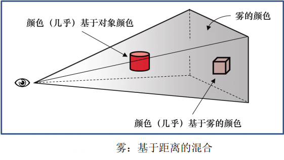
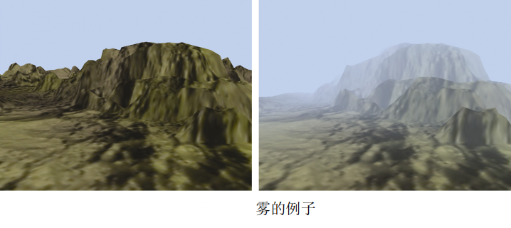
There are many methods to simulate fog, from very simple model to complex model including light scattering effect. Even very simple methods are effective. One way is to mix the actual pixel color with another color (the color of fog is usually gray or bluish gray - also used for background color) based on the distance of the object from the eye.
The following figure illustrates this concept. The eye (camera) is displayed on the left, and two red objects are placed in the viewing cone. The cylinder is closer to the eye, so it is mainly the original color (red); the cube is far away from the eye, so it is mainly fog. For this simple implementation, almost all calculations can be performed in the fragment shader.
The following program shows the relevant code of a very simple fog algorithm, which uses the linear mixing from object color to fog color according to the distance from camera to pixel. Specifically, this example adds fog to the height map example in the previous program "✠ OpenGL-10-enhanced surface detail".
// Vertex Shader
#version 430
...
out vec3 vertEyeSpacePos;
...
// Calculates the vertex position in visual space regardless of perspective and sends it to the clip shader
// The variable p is the vertex after height mapping, as described in "✠ OpenGL-10-enhanced surface detail"
vertEyeSpacePos = (mv_matrix * p).xyz;

// Fragment Shader
#version 430
...
in vec3 vertEyeSpacePos;
out vec4 fragColor;
...
void main() {
	vec4 fogColor = vec4(0.7, 0.8, 0.9, 1.0);// Blue grey
	float fogStart = 0.2;
	float fogEnd = 0.8;
	// In visual space, the distance from the camera to the vertex is the length of the vector to the vertex,
	// Because of the (0,0,0) position of the camera in visual space
	float dist = length(vertEyeSpacePos.xyz);
	float fogFactor = clamp((fogEnd-dist)/(fogEnd-fogStart), 0.0, 1.0);
	fragColor = mix(fogColor, texture(t, tc), fogFactor);
}
The clamp() function of GLSL is used to limit this ratio to values between 0.0 and 1.0. Then, GLSL's mix() function
Returns a weighted average of fog color and object color based on the value of fogFactor.
genFType clamp(genFType x, genFType minVal, genFType maxVal)
return: min(max(x, minVal), maxVal). That is, the final result∈[minVal,maxVal]
If minVal > maxVal,The result is unknown.

genFType mix(genFType x, genFType y, genFType a)
return: x And y Linear mixing of, e.g x·(1-a)+y·a
Let dist=0.1, then (0.8-0.1) / (0.8-0.2) = 1.17 > 1, so fogFactor=1, fragColor=texture(t,tc), that is, the pixel is not in the fog, and the pixel color is the color of the texture.
Let dist=0.7, then (0.8-0.7) / (0.8-0.2) = 0.17, so fogFactor=0.17, fragColor=0.83 × fogColor+0.17 × texture(t,tc), that is, the pixel color is close to the color of the fog.
Let dist > = 0.8, then fogFactor=0, fragColor=fogColor, that is, the pixel color is the fog color, and the pixel cannot be seen.
Compound, blend, transparency
Recall that "✠ OpenGL-2-image pipeline". The pixel operation uses Z buffer. When another object is found closer to the pixel, the hidden surface is eliminated by replacing the existing pixel color. We can actually control this process better - we can choose to mix two pixels.
When a pixel is rendered, it is called a "source" pixel. Pixels that are already in the frame buffer (possibly rendered from previous objects) are called "targets" Pixels. OpenGL provides many options to decide which of the two pixels or their combination will eventually be placed in the frame buffer. Note that the pixel steps are not programmable -- so the OpenGL tool for configuring the desired synthesis can be found in C + + applications, not in shaders.
The two OpenGL functions used to control composition are glBlendEquation(mode) and glblendfunc (SRC factor, destfactor). The following figure shows an overview of the synthesis process.
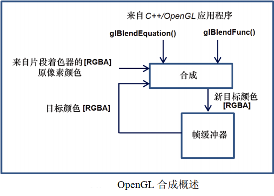
The working process of the synthesis process is as follows:
(1) The source and target pixels are multiplied by the source and target factors, respectively. The source and target factors are specified in the blendFunc() function call.
(2) The modified source and target pixels are then combined using the specified blendEquation to generate a new target color. The mixing equation is specified in the glBlendEquation() call.
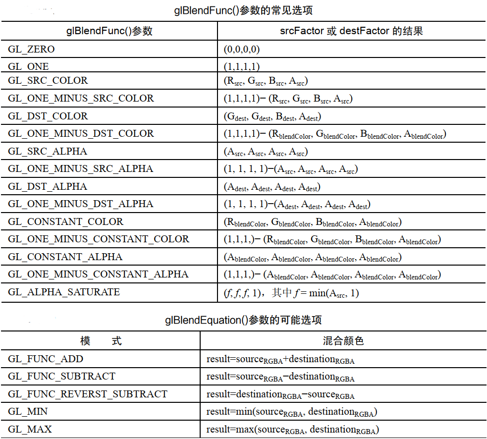
Those options that use "blendColor" require an additional tone glBlendColor() to specify the constant color that will be used to calculate the result of the blend function. There are other blend functions that are not shown in the table.
glBlendFunc() sets srcFactor to GL by default_ One (1.0), destFactor is GL_ZERO(0.0). The default value of glBlendEquation() is GL_FUNC_ADD. Therefore, by default, the source pixel remains unchanged (multiplied by 1), the target pixel is scaled down to 0, and the addition of the two means that the source pixel becomes the color of the frame buffer.
There are also commands glEnable(GL_BLEND) and glDisable(GL_BLEND), which can be used to tell OpenGL to apply the specified blend or ignore it.
We won't explain the effects of all options here, but we'll introduce some illustrative examples. Suppose we specify the following settings in the C++/OpenGL application:
glBlendFunc(GL_SRC_ALPHA, GL_ONE_MINUS_SRC_ALPHA);
glBlendEquation(GL_FUNC_ADD);
The synthesis will proceed as follows:
(1) The source pixel is scaled by its Alpha value.
(2) The target pixel is scaled by 1 − srcaalpha (source transparency).
(3) Pixel values are added together.
For example, if the source pixel is red, it has a 75% opacity, i.e. [1,0,0.75], and the target pixel contains a full color
Opaque green, i.e. [0,1,0,1], the result in the frame buffer will be:
srcPixel * srcAlpha = [0.75, 0, 0, 0.5625]
destPixel * (1-srcAlpha) = [0, 0.25, 0, 0.25]
resulting pixel = [0.75, 0.25, 0, 0.8125]
In other words, it is mainly red, some are green, and it is basically solid color. The overall effect of this setting is that the target pixel is displayed in an amount corresponding to the transparency of the source pixel. In this example, the pixels in the frame buffer are green, the input pixels are red, and the transparency is 25% (opacity is 75%). Therefore, some green is allowed to be displayed in red.
It has been proved that these settings of mixed functions and mixed equations work well in many cases. We apply them to practical examples in a scene containing two 3D models: a torus and a pyramid in front of the torus. The following figure shows a scene with an opaque pyramid on the left and a pyramid on the right. The Alpha value of the pyramid is set to 0.8. Lighting has been added.
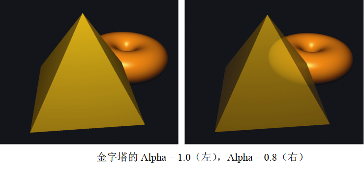
The above effect has obvious shortcomings. Although the pyramid model is now actually transparent, the actually transparent pyramid should show not only the objects behind it, but also its own back.
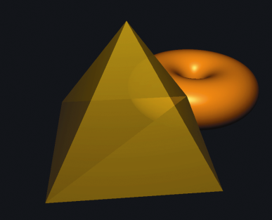
In fact, the reason why the back of the pyramid does not appear is that we have enabled back culling. A reasonable idea might be to disable back culling when drawing pyramids. However, this usually produces other artifacts, as shown in the following figure. The problem with simply disabling backface culling is that the effect of blending depends on the order in which the surface is rendered (because it determines the source and target pixels), and we are not always able to control the rendering order. It is usually advantageous to render opaque objects first and objects later (for example, torus), and finally render the transparent object. This also applies to the surface of the pyramid, and in this case, the two triangles including the bottom of the pyramid look different because one of them is rendered before the front of the pyramid and the other is rendered after. Artifacts such as this are sometimes referred to as "order" Artifacts, and they can be displayed in transparent models because we can not always predict the order in which their triangles will be rendered.
We can solve the problem in the pyramid example by rendering the front and back respectively from the back. The following program shows the code to do this. We specify the Alpha value of the pyramid by unifying variables and pass it to the shader program, and then apply it to the clip shader by replacing the specified Alpha with the calculated output color.
Note that for lighting to work properly, we must flip the normal vector when rendering the back. We do this by sending a flag to the vertex shader, where we flip the normal vector.
void display() {
	...
	aLoc = glGetUniformLocation(renderingProgram, "alpha");
	fLoc = glGetUniformLocation(renderingProgram, "flipNormal");
	...
	glEnable(GL_CULL_FACE);
	...
	glEnable(GL_BLEND);// Configure blend settings
	glBlendFunc(GL_SRC_ALPHA, GL_ONE_MINUS_SRC_ALPHA);
	glBlendEquation(GL_FUNC_ADD);

	glCullFace(GL_FRONT);// Eliminate the front, that is, render the back of the pyramid first
	glProgramUniform1f(renderingProgram, aLoc, 0.3f);// The back is very transparent
	glProgramUniform1f(renderingProgram, fLoc, -1.0f);// Flip back normal
	glDrawArrays(GL_TRIANGLES, 0, numPyramidVertices);

	glCullFace(GL_BACK);// Then render the front of the pyramid
	glProgramUniform1f(renderingProgram, aLoc, 0.7f);// Slightly transparent front
	glProgramUniform1f(renderingProgram, fLoc, 1.0f);// The front does not need to flip the normal vector
	glDrawArrays(GL_TRIANGLES, 0, numPyramidVertices);

	glDisable(GL_BLEND);
}
// Vertex Shader
#version 430
...
if (flipNormal < 0)
	varyingNormal = -varyingNormal;
...

// Fragment Shader
#version 430
...
fragColor = globalAmbient*material.ambient + ... etc.// Same as Blinn phone lighting
fragColor = vec4(fragColor.xyz, alpha);// Replace with the alpha value sent by the unified variable
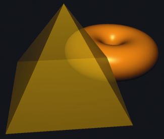
The results of this "two pass correction" solution are shown in the figure below:
Although it works well here, the two pass solution shown in the above program is not always sufficient. For example, some more complex models may have front facing hidden surfaces, and if such objects become transparent, our algorithm will not be able to render those hidden forward parts of the model. Alec Jacobson describes a five pass sequence applicable to a large number of cases [A. Jacobson, "check tricks for OpenGL transparency," 2012, accessed October 2018.].
User defined clipping plane
OpenGL can be applied not only to visual cones, but also to specify clipping planes. One use of user-defined clipping planes is to slice a model. This allows you to create complex shapes by starting with a simple model and slicing from it.
The clipping plane is defined using the standard mathematical definition of the plane: ax + by + cz + d = 0
Where a, b, C and D are parameters used to define a specific plane in 3D space with X, Y and Z axes. The parameter represents the vector (a,b,c) perpendicular to the plane and the distance d from the origin to the plane.
You can use vec4 to specify such a plane in the vertex shader as follows:
vec4 clip_plane = vec4(0.0, 0.0, -1.0, 0.2);
This corresponds to the plane: (0.0) x + (0.0) y + (-1.0) z + 0.2 = 0
Then, by using the built-in GLSL variable gl_ClipDistance [], clipping can be realized in vertex shader, as shown in the following example:
gl_ClipDistance[0] = dot(clip_plane.xyz, vertPos) + clip_plane.w;
Among them, vertPos refers to attributes at vertices (for example, from VBO), the vertex position entering the vertex shader is defined as above. Then we calculate the signed distance from the clipping plane to the incoming vertex, which is 0 if the vertex is on the plane, or negative or positive depending on which side of the plane the vertex is on. The subscript of gl_ClipDistance array allows multiple clipping distances to be defined (i.e. multiple planes). The maximum number of user clipping planes that can be defined depends on the OpenGL implementation of the graphics card.
User defined clipping must then be enabled in the C++/OpenGL application. Built in OpenGL identifier_ CLIP_ DISTANCE0, GL_CLIP_DISTANCE1, etc., corresponding to each gl_ClipDistance [] array element.
For example, turn on the 0th user-defined clipping plane, as shown below.
glEnable(GL_CLIP_DISTANCE0);
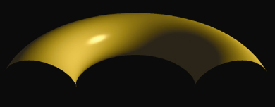
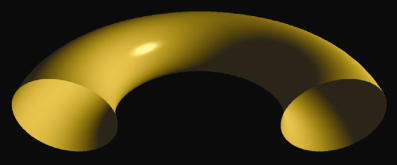
Applying the previous steps to our luminous torus produces the output shown in the following figure, where the first half of the torus has been clipped (rotation has also been applied to provide a clearer view).
It may look as if the bottom of the torus has also been trimmed, but this is because the inner surface of the torus is not rendered. When clipping will show the inner surface of the shape, you also need to render them, otherwise the model will display incompletely.
Rendering the inner surface requires calling GL again_ Drawarrays() and reverse the winding order. In addition, when rendering back triangles, you must reverse the surface normal vector.
void display() {
	...
	flipLoc = glGetUniformLocation(renderingProgram, "flipNormal");
	...
	glEnable(GL_CLIP_DISTANCE0);// Enable the 0th user-defined clipping plane
	// Draw the outer surface normally
	glUniform1i(flipLoc, 0);
	glFrontFace(GL_CCW);
	glDrawElements(GL_TRIANGLES, numTorusIndices, GL_UNSIGNED_INT, 0);
	// Render back, normal vector inversion
	glUniform1i(flipLoc, 1);
	glFrontFace(GL_CW);
	glDrawElements(GL_TRIANGLES, numTorusIndices, GL_UNSIGNED_INT, 0);
}
// Vertex Shader
#version 430
...
vec4 clip_plane = vec4(0.0, 0.0, -1.0, 0.5);
uniform int flipNormal;// Flag of reverse normal vector
...
void main() {
	...
	if (flipNormal == 1)
		varyingNormal = -varyingNormal;
	...
	// Calculates the signed distance from the clipping plane to the incoming vertex
	gl_ClipDistance[0] = dot(clip_plane.xyz, vertPos) + clip_plane.w;
	...
}
3D texture
The 2D texture contains image data indexed by two variables, while the 3D texture contains the same type of image data, but is in a 3D structure indexed by three variables. The first two dimensions still represent the width and height in the texture map, and the third dimension represents the depth.
It is suggested to treat the 3D texture as a substance, and we immerse (or "immerse") the textured object, so that the surface points of the object can obtain color from the corresponding positions in the texture. Alternatively, it can be imagined that the object is "carved" from the 3D texture "Cube", just like a sculptor carves a character from a solid marble.
3D textures are usually generated programmatically. According to the colors in the texture, we can build a three-dimensional array containing these colors. If the texture contains "patterns" that can be used with various colors, we may build an array of patterns, such as 0 and 1.
void generate3Dpattern() {
	for (int x = 0; x < texWidth; x++) {
		for (int y = 0; y < texHeight; y++) {
			for (int z = 0; z < texDepth; z++) {
				if ((y / 10) % 2 == 0)
					tex3Dpattern[x][y][z] = 0.0;
				else
					tex3Dpattern[x][y][z] = 1.0;
			}
		}
	}
}
The patterns generated by the above program and stored in the tex3Dpattern array are as follows: (0 is blue and 1 is yellow)
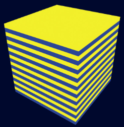
When y=[0-9] or [20-29] or [40-49]... tex3Dpattern=0;
When y=[10-19] or [30-39] or [50-59]... tex3Dpattern=1;
Thus, a blue and yellow 3D pattern related only to the y-axis is generated.
Similarly, if 3D chessboard texture is generated, the algorithm is as follows:
void generate3Dpattern() {
	int xStep, yStep, zStep, sumSteps;
	for (int x = 0; x < texWidth; x++) {
		for (int y = 0; y < texHeight; y++) {
			for (int z = 0; z < texDepth; z++) {
				xStep = (x / 10) % 2;
				yStep = (y / 10) % 2;
				zStep = (z / 10) % 2;
				sumSteps = xStep + yStep + zStep;
				if (sumSteps % 2 == 0)
					tex3Dpattern[x][y][z] = 0.0;
				else
					tex3Dpattern[x][y][z] = 1.0;
			}
		}
	}
}
To texture an object with a stripe pattern, you need to perform the following steps:
(1) Generate the pattern as shown in the above figure;
(2) An array of bytes using the desired color for the hatch;
(3) Load the byte array into the texture object;
(4) Determine the appropriate 3D texture coordinates of the object vertices;
(5) Use the appropriate sampler in the clip shader to texture the object.
The texture coordinate range of 3D texture is [0... 1], which is the same as that of 2D texture.
In most cases, we want the object to reflect the texture pattern as if it were "carved" (or immersed in it). So the vertex position itself is the texture coordinates! Usually all we need is to apply some simple scaling to ensure that the position coordinates of the object's vertices are mapped to the range of 3D texture coordinates [0,1].
. . .
const int texHeight= 200;
const int texWidth = 200;
const int texDepth = 200;
double tex3Dpattern[texWidth][texHeight][texDepth];
. . .
// Fill the byte array with blue and yellow RGB values according to the pattern built by generate3Dpattern()
void fillDataArray(GLubyte data[ ]) {
	for (int i=0; i<texWidth; i++) {
		for (int j=0; j<texHeight; j++) {
			for (int k=0; k<texDepth; k++) {
				if (tex3Dpattern[i][j][k] == 1.0) {
// yellow
data[i*(texWidth*texHeight*4) + j*(texHeight*4)+ k*4+0]=(GLubyte) 255;// red
data[i*(texWidth*texHeight*4) + j*(texHeight*4)+ k*4+1]=(GLubyte) 255;// green
data[i*(texWidth*texHeight*4) + j*(texHeight*4)+ k*4+2]=(GLubyte) 0;// blue
data[i*(texWidth*texHeight*4) + j*(texHeight*4)+ k*4+3]=(GLubyte) 255;// alpha
				} else {
// blue
data[i*(texWidth*texHeight*4) + j*(texHeight*4)+ k*4+0]=(GLubyte) 0;// red
data[i*(texWidth*texHeight*4) + j*(texHeight*4)+ k*4+1]=(GLubyte) 0;// green
data[i*(texWidth*texHeight*4) + j*(texHeight*4)+ k*4+2]=(GLubyte) 255;// blue
data[i*(texWidth*texHeight*4) + j*(texHeight*4)+ k*4+3]=(GLubyte) 255;// alpha
} } } }
// Build a 3D pattern of stripes
void generate3Dpattern() {
	for (int x=0; x<texWidth; x++) {
		for (int y=0; y<texHeight; y++) {
			for (int z=0; z<texDepth; z++) {
				if ((y/10)%2 == 0)
					tex3Dpattern[x][y][z] = 0.0;
				else
					tex3Dpattern[x][y][z] = 1.0;
} } } }
// Loads an array of sequential byte data into a texture object
int load3DTexture() {
	GLuint textureID;
	GLubyte* data = new GLubyte[texWidth*texHeight*texDepth*4];
	fillDataArray(data);
	glGenTextures(1, &textureID);
	glBindTexture(GL_TEXTURE_3D, textureID);
	glTexParameteri(GL_TEXTURE_3D, GL_TEXTURE_MIN_FILTER, GL_LINEAR);
	glTexStorage3D(GL_TEXTURE_3D, 1, GL_RGBA8, texWidth, texHeight, texDepth);
	glTexSubImage3D(GL_TEXTURE_3D, 0, 0, 0, 0, texWidth, texHeight, texDepth,
GL_RGBA, GL_UNSIGNED_INT_8_8_8_8_REV, data);
	return textureID;
}
void init(GLFWwindow* window) {
	. . .
	generate3Dpattern(); // 3D patterns and textures are loaded only once, so they are made in init()
	stripeTexture = load3DTexture(); // Save integer pattern ID for 3D texture
}
void display(GLFWwindow* window, double currentTime) {
	. . .
	glActiveTexture(GL_TEXTURE0);
	glBindTexture(GL_TEXTURE_3D, stripeTexture);
	glDrawArrays(GL_TRIANGLES, 0, numObjVertices);
}
########################################################
// Vertex Shader
. . .
out vec3 originalPosition;// The original model vertices will be used for texture coordinates
. . .
void main(void) {
	originalPosition = position;// Transfer the original model coordinates as 3D texture coordinates
	gl_Position = proj_matrix * mv_matrix * vec4(position,1.0);
}

// Fragment Shader
. . .
in vec3 originalPosition;// Accept the original model coordinates as 3D texture coordinates
out vec4 fragColor;
. . .
layout (binding=0) uniform sampler3D s;
void main(void) {
	// The vertex range is [− 1, + 1], and the conversion to texture coordinate range is [0,1]
	fragColor = texture(s, originalPosition / 2.0 + 0.5);
}
In the application, the load3Dtexture() function loads the generated data into the 3D texture. Instead of using SOIL2 to load textures, it makes related OpenGL calls directly. The image data should be formatted as a byte sequence corresponding to the RGBA color component. The function fillDataArray() performs this operation, applying yellow and blue RGB values based on the strip pattern built by the generate3Dpattern() function and saved in the tex3Dpattern array. Also note that the texture type GL is specified in the display() function_ TEXTURE_ 3D.
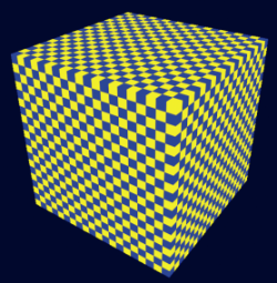
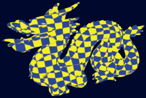
Since we want to use the object's vertex positions as texture coordinates, we pass them from the vertex shader to the clip shader. The clip shader scales them so that they are mapped to the range [0, 1] according to the criteria of texture coordinates. Finally, the 3D texture is accessed through the sampler3D unified variable, which takes three parameters instead of two. We use the original X, Y, and Z coordinates of the vertices and zoom to the correct range to access the texture. The results are shown in the figure below.

If you use chessboard 3D texture, the effect is as follows:
Noise
Randomness or noise can be used to simulate many natural phenomena. A common technique is Perlin noise, which is named after Ken Perlin.
There are many noise applications in graphic scenes. Some common examples are clouds, topography, wood grain, minerals (such as veins in marble), smoke, combustion, flames, planetary surfaces, and random motion.
A collection of spatial data containing noise, such as 2D or 3D, is sometimes referred to as a noise map.
#include<random>
...
double noise[noiseWidth][noiseHeight][noiseDepth];
...
void generateNoise() {
	for (int x = 0; x < noiseWidth; x++)
		for (int y = 0; y < noiseHeight; y++)
			for (int z = 0; z < noiseDepth; z++)
				// Calculate a double type value in the range of [0... 1]
				noise[x][y][z] = (double) rand() / (RAND_MAX + 1);
}
Next, the fillDataArray() function to copy the noise data into the byte array for loading into the texture object.
void fillDataArray(GLubyte data[]) {
	for (int i = 0; i < noiseWidth; i++) {
		for (int j = 0; j < noiseHeight; j++) {
			for (int k = 0; k < noiseDepth; k++) {
				data[i*(noiseWidth*noiseHeight*4)+j*(noiseHeight*4)+k*4+0] =
											(GLubyte) (noise[i][j][k] * 255);
				data[i*(noiseWidth*noiseHeight*4)+j*(noiseHeight*4)+k*4+1] =
											(GLubyte) (noise[i][j][k] * 255);
				data[i*(noiseWidth*noiseHeight*4)+j*(noiseHeight*4)+k*4+2] =
											(GLubyte) (noise[i][j][k] * 255);
				data[i*(noiseWidth*noiseHeight*4)+j*(noiseHeight*4)+k*4+3] =
																(GLubyte) 25;
}}}}
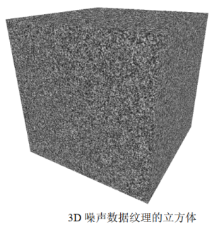
Let's make noiseHeight=noiseWidth=noiseDepth=256, the others are the same as the previous example code, and the effect is as follows:
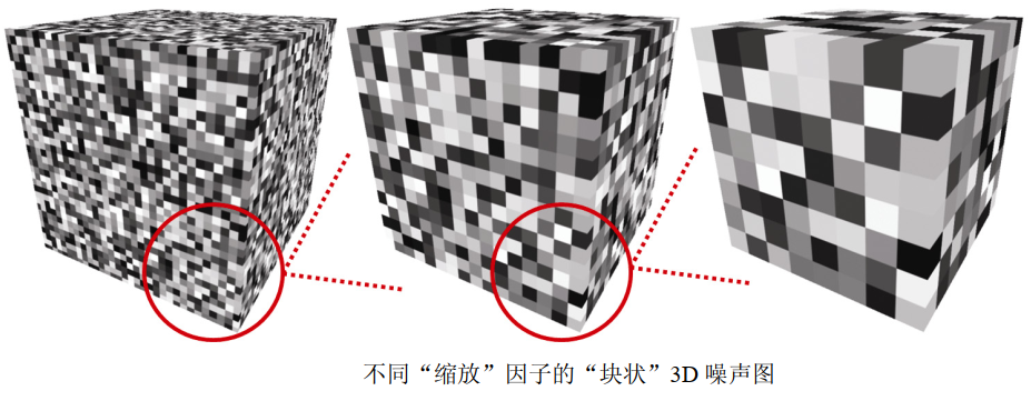
Depending on the scale factor used for the division index, the resulting 3D texture can appear more or less "blocky". In the following image, the texture shows the result of magnification, dividing the index by scaling factors 8, 16, and 32 (from left to right).
void fillDataArray(GLubyte data[]) {
	int zoom = 8;// Scaling factor
	for (int i=0; i<noiseWidth; i++) {
		for (int j=0; j<noiseHeight; j++) {
			for (int k=0; k<noiseDepth; k++) {
				data[i*(noiseWidth*noiseHeight*4)+j*(noiseHeight*4)+k*4+0] =
						(GLubyte) (noise [i/zoom] [j/zoom] [k/zoom] * 255);
				data[i*(noiseWidth*noiseHeight*4)+j*(noiseHeight*4)+k*4+1] =
						(GLubyte) (noise [i/zoom] [j/zoom] [k/zoom] * 255);
				data[i*(noiseWidth*noiseHeight*4)+j*(noiseHeight*4)+k*4+2] =
						(GLubyte) (noise [i/zoom] [j/zoom] [k/zoom] * 255);
				data[i*(noiseWidth*noiseHeight*4)+j*(noiseHeight*4)+k*4+3] =
																(GLubyte) 255;
} } } }
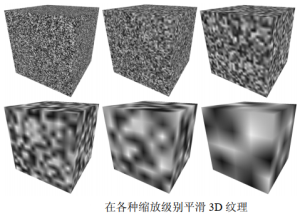
By interpolating from each discrete gray color value to the next gray color value, we can smooth the "block effect" in a specific noise image. That is, for each small "block" in a given 3D texture, we set the color of each texture element in the block by interpolating from its color to the color of its adjacent blocks. The interpolation code is in the function smoothNoise() shown below. The following figure shows the resulting "smooth" texture (scaling factors 2, 4, 8, 16, 32 and 64 - left to right, top to bottom). Note that the scaling factor is now a double type quantity, because we need a decimal component to determine the interpolated gray value of each texture.
double smoothNoise(double x1, double y1, double z1) {
	// Fraction of x1, y1, and z1 (percentage from current block to next block for current morpheme)
	double fractX = x1 - (int) x1;
	double fractY = y1 - (int) y1;
	double fractZ = z1 - (int) z1;
	// Index of adjacent pixels in X, Y, and Z directions
	int x2 = ((int)x1 + noiseWidth + 1) % noiseWidth;
	int y2 = ((int)y1 + noiseHeight + 1) % noiseHeight;
	int z2 = ((int)z1 + noiseDepth + 1) % noiseDepth;
	// The noise is smoothed by interpolating the gray level according to three axis directions
	double value = 0.0;
	value += (1-fractX)*(1-fractY)*(1-fractZ)*noise[(int)x1][(int)y1][(int)z1];
	value += (1-fractX)*fractY*(1-fractZ)*noise[(int)x1][(int)y2][(int)z1];
	value += fractX*(1-fractY)*(1-fractZ)*noise[(int)x2][(int)y1][(int)z1];
	value += fractX*fractY*(1-fractZ)*noise[(int)x2][(int)y2][(int)z1];
	value += (1-fractX)*(1-fractY)*fractZ *noise[(int)x1][(int)y1][(int)z2];
	value += (1-fractX)*fractY*fractZ*noise[(int)x1][(int)y2][(int)z2];
	value += fractX*(1-fractY)*fractZ*noise[(int)x2][(int)y1][(int)z2];
	value += fractX*fractY *fractZ *noise[(int)x2][(int)y2][(int)z2];
	return value;
}

double turbulence(double x, double y, double z, double size) {
	double value = 0.0, initialSize = size;
	while (size >= 0.9) {
		value = value + smoothNoise(x / size, y / size, z / size) * size;
		size = size / 2.0;
	}
	value = 128.0 * value / initialSize;
	return value;
}

double logistic(double x) {
	double k = 3.0;
	return (1.0 / (1.0 + pow(2.718, -k*x)));
}

void fillDataArray(GLubyte data[]) {
	double veinFrequency = 1.75;
	double turbPower = 3.0;  //4
	double turbSize = 32.0;
	for (int i = 0; i<noiseHeight; i++) {
		for (int j = 0; j<noiseWidth; j++) {
			for (int k = 0; k<noiseDepth; k++) {
				double xyzValue = (float)i / noiseWidth + (float)j / noiseHeight + (float)k / noiseDepth + turbPower * turbulence(i, j, k, turbSize) / 256.0;
				double sineValue = logistic(abs(sin(xyzValue * 3.14159 * veinFrequency)));
				sineValue = max(-1.0, min(sineValue*1.25 - 0.20, 1.0));

				float redPortion = 255.0f * (float)sineValue;
				float greenPortion = 255.0f * (float)min(sineValue*1.5 - 0.25, 1.0);
				float bluePortion = 255.0f * (float)sineValue;

				data[i*(noiseWidth*noiseHeight * 4) + j*(noiseHeight * 4) + k * 4 + 0] = (GLubyte)redPortion;
				data[i*(noiseWidth*noiseHeight * 4) + j*(noiseHeight * 4) + k * 4 + 1] = (GLubyte)greenPortion;
				data[i*(noiseWidth*noiseHeight * 4) + j*(noiseHeight * 4) + k * 4 + 2] = (GLubyte)bluePortion;
				data[i*(noiseWidth*noiseHeight * 4) + j*(noiseHeight * 4) + k * 4 + 3] = (GLubyte)255;
			}
		}
	}
}
The smoothNoise() function calculates the gray value of each texture element in the smooth version of a given noise image by calculating the weighted average of 8 gray values around the texture element in the corresponding original "block" noise image. That is, it averages the color values at the 8 vertices of the small "block" where the texture element is located. The weight of each of these "neighbor" colors is based on the distance between the texture element and each neighbor and normalized to the range [0... 1].
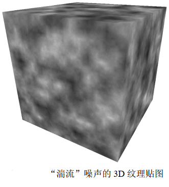
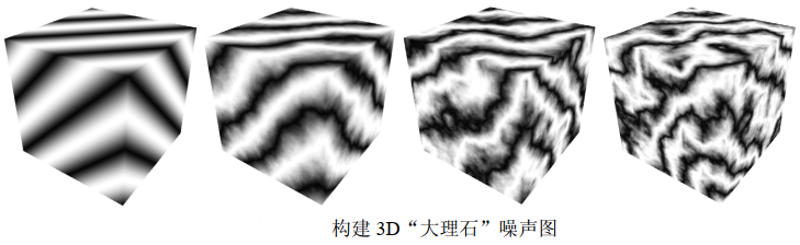
Next, smooth noise maps of various scaling factors are combined. Create a new noise graph, where each texture element is formed by another weighted average, this time based on the sum of texture elements at the same position in each "smooth" noise graph, where the scaling factor is used as the weight. This effect is called "turbulence" by Perlin, although it is actually more closely related to the harmonics generated by summing various waveforms. The new turbulence() function and the modified version of fillDataArray() specify a noise graph that sums the scaling levels 1 to 32 (powers of 2), as shown below. It also shows the mapping results of the noise graph generated on the cube.
double turbulence(double x, double y, double z, double maxZoom) {
	double sum = 0.0, zoom = maxZoom;
	while (zoom >= 1.0) {// The last time is when zoom = 1
		// Calculate the weighted sum of the smoothed noise map
		sum = sum + smoothNoise(x / zoom, y / zoom, z / zoom) * zoom;
		zoom = zoom / 2.0; // Scaling factor for each power of 2
	}
	sum = 128.0 * sum / maxZoom; // For maxZoom value not greater than 64, ensure RGB < 256
	return sum;
}

void fillDataArray(GLubyte data[ ] ) {
	double maxZoom = 32.0;
	for (int i=0; i<noiseWidth; i++) {
		for (int j=0; j<noiseHeight; j++) {
			for (int k=0; k<noiseDepth; k++) {
			data[i*(noiseWidth*noiseHeight*4)+j*(noiseHeight*4)+k*4+0] =
								(GLubyte) turbulence(i, j, k, maxZoom);
			data[i*(noiseWidth*noiseHeight*4)+j*(noiseHeight*4)+k*4+1] =
								(GLubyte) turbulence(i, j, k, maxZoom);
			data[i*(noiseWidth*noiseHeight*4)+j*(noiseHeight*4)+k*4+2] =
								(GLubyte) turbulence(i, j, k, maxZoom);
			data[i*(noiseWidth*noiseHeight*4)+j*(noiseHeight*4)+k*4+3] =
															(GLubyte) 255;
} } } }
Noise application - marble
By modifying the noise map and adding Phong lighting with appropriate ADS materials, we can make the Dragon model look like a marble stone.
We first generate a stripe pattern, which is somewhat similar to the "stripe" example earlier in this chapter - the new stripes are different from the previous stripes, first because they are diagonal and because they are generated by sine waves, so the edges are blurred. Then, we use the noise map to disturb these lines and store them as gray values. The fillDataArray() function is changed as follows:
void fillDataArray(GLubyte data[ ]) {
	double veinFrequency = 2.0;
	double turbPower = 1.5;
	double maxZoom = 64.0;
	for (int i=0; i<noiseWidth; i++) {
		for (int j=0; j<noiseHeight; j++) {
			for (int k=0; k<noiseDepth; k++) {
					double xyzValue = (float)i / noiseWidth + (float)j / noiseHeight + (float)k / noiseDepth +
																turbPower * turbulence(i,j,k,maxZoom) / 256.0;
					double sineValue = abs(sin(xyzValue * 3.14159 * veinFrequency));
					float redPortion = 255.0f * (float)sineValue;
					float greenPortion = 255.0f * (float)sineValue;
					float bluePortion = 255.0f * (float)sineValue;
					data[i*(noiseWidth*noiseHeight*4)+j*(noiseHeight*4)+k*4+0] = (GLubyte) redPortion;
					data[i*(noiseWidth*noiseHeight*4)+j*(noiseHeight*4)+k*4+1] = (GLubyte) greenPortion;
					data[i*(noiseWidth*noiseHeight*4)+j*(noiseHeight*4)+k*4+2] = (GLubyte) bluePortion;
					data[i*(noiseWidth*noiseHeight*4)+j*(noiseHeight*4)+k*4+3] = (GLubyte) 255;
} } } }
The variable veinFrequency is used to adjust the number of stripes, and turbSize adjusts the scaling factor used when generating turbulence, turbPower adjusts the amount of disturbance in the fringe (set it to 0 so that the fringe is not disturbed). Since the same sine wave value is used for all 3 (RGB) color components, the final color stored in the image data array is grayscale. The following figure shows the resulting texture map of various turbPower values (0.0, 5.5, 1.0 and 1.5, from left to right).
Because we want the marble to have a shiny appearance, we use Phong shading to make the "marble" texture object look convincing. The preceding program summarizes the code for generating marble dragon. In addition to passing the original vertex coordinates as 3D texture coordinates (as described earlier), vertex and fragment shaders are the same as those used for Phong shading. Fragment shaders combine noise results with lighting results using the techniques described in the previous code.
// White ADS settings for Phong shading
...
float globalAmbient[4] = {0.5f, 0.5f, 0.5f, 1.0f};
float lightAmbient[4] = {0.0f, 0.0f, 0.0f, 1.0f};
float lightDiffuse[4] = {1.0f, 1.0f, 1.0f, 1.0f};
float lightSpecular[4] = {1.0f, 1.0f, 1.0f, 1.0f};
float matShi = 75.0f;

void init(GLFWwindow* window) {
	. . .
	generateNoise();
	noiseTexture = load3DTexture(); // Like the previous program, it is responsible for calling fillDataArray()
}
void fillDataArray(GLubyte data[]) {
	double veinFrequency = 1.75;
	double turbPower = 3.0;
	double turbSize = 32.0;
	// The rest of the construction of the marble noise diagram is the same as before
	. . .
}
// Vertex shader, as before
// Fragment Shader
. . .
void main(void) {
	. . .
	// Model vertex value [- 1.5, + 1.5], texture coordinate value [0, 1]
	vec4 texColor = texture(s, originalPosition / 3.0 + 0.5);
	fragColor = 0.7 * texColor * (globalAmbient + light.ambient + light.diffuse * max(cosTheta,0.0))
								+ 0.5 * light.specular * pow(max(cosPhi, 0.0), material.shininess);
}
There are many ways to simulate different colors of marble (or other stones). One way to change the Color of the "vein" in marble is to modify the definition of the Color variable in the fillDataArray() function, for example, by adding a green component:
float redPortion = 255.0f * (float)sineValue;
float greenPortion = 255.0f * (float)min(sineValue*1.5 - 0.25, 1.0);
float bluePortion = 255.0f * (float)sineValue;
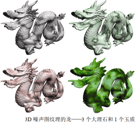
We can also introduce ADS material value [i.e. specified in init()] to simulate completely different types of stones, such as "jade".
The following figure shows four examples. The first three use the settings shown in the example above, and the fourth example uses the "jade" ADS material value.
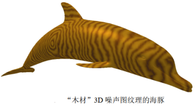
Noise application - wood
Brown hues can be made by combining a similar number of red and green and a small amount of blue. Then we apply Phong shading with low "gloss".
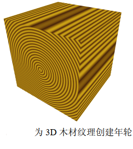
We can modify the fillDataArray() function to generate the growth rings around the Z axis in our 3D texture map, and use the trigonometric function to specify the X and Y values equidistant from the Z axis. We repeat this process using a sine wave cycle, uniformly raising and lowering the red and green components according to this sine wave to produce different brown tones. The variable sineValue maintains a precise tone and can be adjusted by slightly offsetting one component or another (in this case, increase red by 80 and green by 30). We can create more (or fewer) rings by adjusting the value of xyPeriod.
void fillDataArray(GLubyte data[ ]) {
	double xyPeriod = 40.0;
	for (int i=0; i<noiseWidth; i++) {
		for (int j=0; j<noiseHeight; j++) {
			for (int k=0; k<noiseDepth; k++) {
				double xValue = (i - (double)noiseWidth/2.0) / (double)noiseWidth;
				double yValue = (j - (double)noiseHeight/2.0) / (double)noiseHeight;
				double distanceFromZ = sqrt(xValue * xValue + yValue * yValue)
				double sineValue = 128.0 * abs(sin(2.0 * xyPeriod * distanceFromZ * 3.14159));
				float redPortion = (float)(80 + (int)sineValue);
				float greenPortion = (float)(30 + (int)sineValue);
				float bluePortion = 0.0f;
				data[i*(noiseWidth*noiseHeight*4)+j*(noiseHeight*4)+k*4+0] = (GLubyte) redPortion;
				data[i*(noiseWidth*noiseHeight*4)+j*(noiseHeight*4)+k*4+1] = (GLubyte) greenPortion;
				data[i*(noiseWidth*noiseHeight*4)+j*(noiseHeight*4)+k*4+2] = (GLubyte) bluePortion;
				data[i*(noiseWidth*noiseHeight*4)+j*(noiseHeight*4)+k*4+3] = (GLubyte) 255;
} } } }
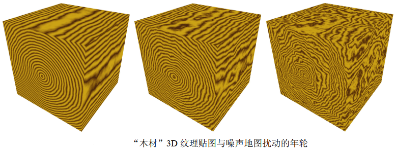
The wooden rings above are a good start, but they don't look very realistic - they're perfect. To improve this, we use the noise map (more specifically, turbulence) to perturb the distanceFromZ variable so that the ring has a slight change. The calculation is modified as follows:
double distanceFromZ =
sqrt(xValue * xValue + yValue * yValue) +
turbPower * turbulence(i, j, k, maxZoom) / 256.0;
Similarly, the variable turbPower adjusts how much turbulence is applied (set it to 0.0 to produce the undisturbed version shown in the above figure), and maxZoom specifies the scaling value (32 in this example). The following figure shows the wood texture obtained by turbPower values of 0.05, 1.0 and 2.0 (from left to right).
We can now apply 3D wood texture mapping to the model. The realism of the texture can be further enhanced by applying rotation to the vertex position of the originalPosition used for texture coordinates, because most items carved with wood are not fully aligned with the direction of the growth rings. To do this, we send an additional rotation matrix to the shader to rotate the texture coordinates. We also added Phong shading with appropriate wood color ADS value and moderate gloss. Let's create a "wooden dolphin":
glm::mat4 texRot;
// Wood (brown)
float matAmbient[4] = {0.5f, 0.35f, 0.15f, 1.0f};
float matDiffuse[4] = {0.5f, 0.35f, 0.15f, 1.0f};
float matSpecular[4] = {0.5f, 0.35f, 0.15f, 1.0f};
float matShi = 15.0f;
void init(GLFWwindow* window) {
	. . .
	// Rotation applied to texture coordinates - adds additional grain variation
	texRot = glm::rotate(glm::mat4(1.0f), toRadians(20.0f), glm::vec3(0.0f, 1.0f, 0.0f));
}
void fillDataArray(GLubyte data[ ]) {
	double xyPeriod = 40.0;
	double turbPower = 0.1;
	double maxZoom = 32.0;
	for (int i=0; i<noiseWidth; i++) {
		for (int j=0; j<noiseHeight; j++) {
			for (int k=0; k<noiseDepth; k++) {
				double xValue = (i - (double)noiseWidth/2.0) / (double)noiseWidth;
				double yValue = (j - (double)noiseHeight/2.0) / (double)noiseHeight;
				double distanceFromZ = sqrt(xValue * xValue + yValue * yValue)
							+ turbPower * turbulence(i, j, k, maxZoom) / 256.0;
				double sineValue = 128.0 * abs(sin(2.0 * xyPeriod * distanceFromZ * Math.PI));
				float redPortion = (float)(80 + (int)sineValue);
				float greenPortion = (float)(30 + (int)sineValue);
				float bluePortion = 0.0f;
				data[i*(noiseWidth*noiseHeight*4)+j*(noiseHeight*4)+k*4+0] = (GLubyte) redPortion;
				data[i*(noiseWidth*noiseHeight*4)+j*(noiseHeight*4)+k*4+1] = (GLubyte) greenPortion;
				data[i*(noiseWidth*noiseHeight*4)+j*(noiseHeight*4)+k*4+2] = (GLubyte) bluePortion;
				data[i*(noiseWidth*noiseHeight*4)+j*(noiseHeight*4)+k*4+3] = (GLubyte) 255;
} } } }
void display(GLFWwindow* window, double currentTime) {
	. . .
	tLoc = glGetUniformLocation(renderingProgram, "texRot");
	glUniformMatrix4fv(tLoc, 1, false, glm::value_ptr(texRot));
	. . .
}
##############################################################
//Vertex Shader
. . .
uniform mat4 texRot;
void main(void) {
	. . .
	originalPosition = vec3(texRot * vec4(position,1.0)).xyz;
	. . .
}

//Fragment Shader
. . .
void main(void) {
	. . .
	uniform mat4 texRot;
	. . .
	// Combine lighting with 3D textures
	fragColor = 0.5 * ( . . . ) + 0.5 * texture(s,originalPosition / 2.0 + 0.5);
}
There is another noteworthy detail in the clip shader. Because we rotate the model within the 3D texture, sometimes the vertex position may move beyond the required [0... 1] texture coordinates due to rotation. If this happens, we can adjust this possibility by dividing the original vertex position by a larger number (for example, 4.0 instead of 2.0), and then add a slightly larger number (for example, 0.6) to center it in texture space.
Noise application - cloud
The "turbulence" noise map constructed earlier looks a bit like a cloud. Of course, it's not the right color, so we first change it from gray to an appropriate mixture of light blue and white. A direct method is to specify a color with a maximum value of 1.0 for the blue component and a variation (but equal) value of 0.0 ~ 1.0 for the red and green components, depending on the value in the noise graph. The new fillDataArray() function is as follows:
void fillDataArray(GLubyte data[ ]) {
	for (int i=0; i<noiseWidth; i++) {
		for (int j=0; j<noiseHeight; j++) {
			for (int k=0; k<noiseDepth; k++) {
				float brightness = 1.0f - (float) turbulence(i,j,k,32) / 256.0f;
				float redPortion = brightness*255.0f;
				float greenPortion = brightness*255.0f;
				float bluePortion = 1.0f*255.0f;
				data[i*(noiseWidth*noiseHeight*4)+j*(noiseHeight*4)+k*4+0] = (GLubyte) redPortion;
				data[i*(noiseWidth*noiseHeight*4)+j*(noiseHeight*4)+k*4+1] = (GLubyte) greenPortion;
				data[i*(noiseWidth*noiseHeight*4)+j*(noiseHeight*4)+k*4+2] = (GLubyte) bluePortion;
				data[i*(noiseWidth*noiseHeight*4)+j*(noiseHeight*4)+k*4+3] = (GLubyte) 255;
} } } }
The generated blue version of the noise map can now be used to texture the sky curtain. Recall that the sky curtain is a sphere or hemisphere that is textured and rendered with the depth test disabled and placed around the camera (similar to the sky box).
One way to build the sky curtain is to use vertex coordinates as texture coordinates and texture it in the same way as we do with other 3D textures. However, in this case, it turns out that using the 2D texture coordinates of the sky curtain will produce a pattern that looks more like a cloud, because the spherical distortion will stretch the texture map slightly. We can get 2D slices from the noise map by setting the third dimension in the texture() call of GLSL to a constant value. Assuming that the texture coordinates of the sky curtain have been sent to the OpenGL pipeline in the vertex attributes in a standard way, the following fragment shader textures it with 2D slices of the noise map:
#version 430
in vec2 tc;
out vec4 fragColor;
uniform mat4 mv_matrix;
uniform mat4 proj_matrix;
layout(binding = 0) uniform sampler3D s;
void main() {
	fragColor = texture(s, vec3(tc.x, tc.y, 0.5));
}
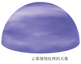
The resulting textured sky curtain is shown in the figure below. Although the camera is usually placed in the sky curtain, we use the camera to render outside, so we can see the effect of the dome itself. The current noise map causes the cloud to "look blurred".
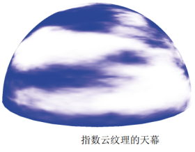
Although our hazy clouds look good, we want to shape them - that is, make them more or less hazy. One method is to modify the turbulence() function to use the exponent (such as logistic function) to make the cloud look more "obvious". The modified turbulence() function and related logistic() functions are shown in the previous program. The complete program also includes the smooth(), fillDataArray() and generateNoise() functions described earlier.
The "logistic" (or "sigmoid") function has an S-shaped curve with asymptotes at both ends. Common examples are hyperbolic tangent function and f(x) = 1/(1+e − x). They are sometimes referred to as "squeeze" functions.
double turbulence(double x, double y, double z, double size) {
	double value = 0.0, initialSize = size, cloudQuant;
	while(size >= 0.9) {
		value = value + smoothNoise(x/size, y/size, z/size) * size;
		size = size / 2.0;
	}
	cloudQuant = 110.0; // Fine tuned cloud quality
	value = value / initialSize;
	value = 256.0 * logistic(value * 128.0 - cloudQuant);
	return value;
}

double logistic(double x) {
	double k = 0.2; // Fine tune cloud obscuration to produce more or less distinct cloud boundaries
	return (1.0 / (1.0 + pow(2.718, -k*x)));
}
The logistic function makes the color more white or blue than a value in between, resulting in a visual effect with more different cloud boundaries. The variable cloudQuant adjusts the relative amount of white (relative to blue) in the noise map, which in turn results in more (or less) white areas (i.e. different clouds) when the logistic function is applied. The resulting sky curtain now has more obvious clouds, as shown in the following figure.
To enhance the realism of clouds, we should make them vivid in the following ways:
(a) Make them move or "drift" over time;
(b) As they drift, they gradually change their shape.
A simple way to "drift" clouds is to slowly rotate the sky curtain. This is not a perfect solution because real clouds tend to drift in a straight line rather than rotate around the observer. However, if the rotation is slow and the cloud is only used to decorate the scene, the effect may be sufficient.
As clouds drift, they gradually change and may seem tricky at first. However, considering the 3D noise map we use for texture cloud, there is actually a very simple and smart way to achieve this effect. Recall that although we built a 3D texture noise map for the cloud, so far we have only used one "slice" of it to intersect with the 2D texture coordinates of the sky curtain (we set the Z coordinate of the texture lookup to a constant value). So far, the rest of the 3D texture has not been used.
Our trick is to replace the constant Z coordinate of texture lookup with a variable that changes gradually over time. That is, when we rotate the sky curtain, we gradually increase the depth variable, resulting in different slices for texture lookup. Recall that when we built a 3D texture map, we applied smoothing to color changes along three axes. Therefore, adjacent slices in the texture map are very similar, but slightly different. Therefore, by gradually changing the Z value in the texture() call, the appearance of the cloud will gradually change.
double rotAmt = 0.0; // The amount of Y-axis rotation used to make the cloud appear to drift
float depth = 0.01f; // The depth search of 3D noise map is used to gradually change the cloud
. . .
void display(GLFWwindow* window, double currentTime) {
	. . .
	// Gradually rotate the sky curtain
	mMat = glm::translate(glm::mat4(1.0f), glm::vec3(domeLocX, domeLocY, domeLocZ);
	rotAmt += 0.02;
	mMat = glm::rotate(mMat, rotAmt, glm::vec3(0.0f, 1.0f, 0.0f));
	// Gradually modify the third texture coordinate to make the cloud change
	dLoc = glGetUniformLocation(program, "d");
	depth += 0.00005f;
	if (depth >= 0.99f)
		depth = 0.01f; // When we reach the end of the texture map, we return to the beginning
	glUniform1f(dLoc, depth);
	. . .
}
#############################
//Fragment Shader
#version 430
in vec2 tc;
out vec4 fragColor;
uniform float d;
layout (binding=0) uniform sampler3D s;
void main(void) {
	fragColor = texture(s, vec3(tc.x, tc.y, d));// Gradually changing "d" replaces the previous constant
}
The effect of gradually changing the drift and animated cloud is as follows:
They drift from right to left on the sky curtain and slowly change shape as they drift.
Noise applications - special effects
void display() {
	...
	tLoc = glGetUniformLocation(renderingProgram, "t");
	threshold += 0.002f;
	glUniform1f(tLoc, threshold);
	...
	glActiveTexture(GL_TEXTURE0);
	glBindTexture(GL_TEXTURE_3D, noiseTexture);
	glActiveTexture(GL_TEXTURE1);
	glBindTexture(GL_TEXTURE_2D, earthTexture);
	...
	glDrawArrays(GL_TRIANGLES, 0, numSphereVertices);
// Fragment Shader
#version 430
in vec2 tc;// The texture coordinates of the current clip
in vec3 origPos;// The original vertex position in the model for accessing 3D textures
...
layout(binding = 0) uniform sampler3D n;// Sampler for noise texture
layout(binding = 1) uniform sampler2D e;// Sampler for earth texture
...
uniform float t;// Threshold for retaining or discarding fragments
void main() {
	float noise = texture(n, origPos).x;// Get noise value from segment
	if (noise > t) {// If the noise value is greater than the current threshold
		fragColor = texture(e, tc);// Render the clip using the earth texture
	} else {
		discard;// Otherwise, discard the clip (do not render)
	}
}
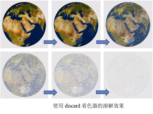
In order to promote the dissolution effect, we introduced the discard command of GLSL. This command is valid only in clip shaders, and when executed, it causes the clip shader to discard the current clip (meaning it is not rendered).
Our strategy is simple. In the C++/OpenGL application, we created a fine-grained noise texture map and a floating-point variable counter that gradually increases over time. This variable is then sent as a unified variable in the shader pipeline, and the noise map is also placed in the texture map with the associated sampler. The fragment shader then uses the sampler to access the noise texture -- in this case, we use the returned noise value to determine whether to discard the fragment. We do this by comparing the gray noise value with the counter, which is used as a "threshold" value. Because the threshold changes gradually over time, we can set it to gradually discard more and more fragments. As a result, the object seems to dissolve gradually.
If possible, the discard command should be used with caution because it may cause performance loss. This is because its existence makes it more difficult for OpenGL to optimize Z-buffer depth testing.
Supplementary notes
The noise map generated in this chapter is based on the program described by Lode Vandevenne. Our 3D cloud generation still has some shortcomings. The texture is not seamless, Therefore, there is an obvious vertical line at the 360 ° point (which is why we start the depth variable with 0.01 instead of 0.0 in the program to avoid encountering seams in the Z dimension of the noise map). If necessary, there is also a simple method to remove seams. Another problem is that at the North peak of the sky curtain, the spherical distortion in the sky curtain will produce a pillow effect.
The clouds we implemented in this chapter also fail to simulate some important aspects of real clouds, such as the way they scatter sunlight. Real clouds tend to be whiter at the top and darker at the bottom. Our cloud also does not achieve the 3D "fluffy" appearance of many actual clouds. Similarly, there are more comprehensive models for generating fog, such as those described by Kilgard and Fernando.
When reading OpenGL documents, readers may notice that GLSL contains some noise functions named noise1(), noise2(), noise3(), and noise4(), which are described as taking input seeds and generating Gaussian like random outputs. We did not use these functions in this chapter because most vendors did not implement them at the time of writing. For example, many NVIDIA graphics cards currently only return a value of 0 for these functions regardless of the input seed.