Article catalogue
1, Theoretical basis
1. Algorithm Introduction
Invasive Weed Optimization (IWO) is a random search bionic optimization algorithm that C.Lucas and A.R.Mehrabian simulated the process of weed diffusion and invasion in nature in 2006. The algorithm is a powerful intelligent optimization algorithm, which has the advantages of easy understanding, good convergence, strong robustness, easy implementation and simple structure. At present, IWO algorithm has been successfully applied in DNA sequence calculation, linear antenna design, power line communication system resource allocation, image recognition, image clustering, constraint engineering design Practical engineering problems such as placement of piezoelectric actuator.
2. Weed characteristics
The most prominent feature of weeds is that seeds are randomly scattered in the field through a variety of transmission ways such as animals, water and wind. Each seed independently uses the resources in the field, finds a suitable growth space, gives full play to its strong adaptability, and makes full use of the resources in the growth environment to obtain sufficient nutrition and grow rapidly. In the process of weed evolution and reproduction, seeds with strong viability reproduce faster and produce more seeds. Conversely, seeds that do not adapt to the environment produce fewer seeds.
2, Case background
1. Problem description
The optimization function of this case is sphere function:
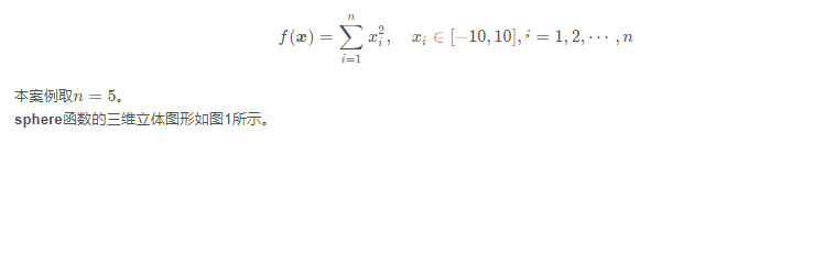
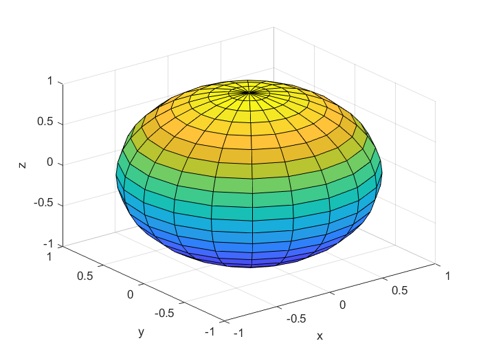
Fig. 1 three dimensional graph of sphere function
2. Problem solving ideas and steps
(1) Initialize population
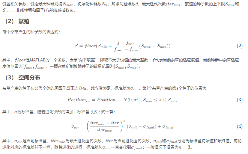
(4) Competitive exclusion rule
The competitive exclusion rule is that after many evolutions, when the population size reaches n Ma x n_ {Max} nmax, sort all individuals according to the fitness value, exclude the individuals with poor fitness and retain the rest. That is, this algorithm first propagates rapidly through weeds to occupy the living space, and then retains the more competitive weeds to continue the spatial search.
3. Algorithm flow
The main steps of IWO algorithm are shown in Figure 2.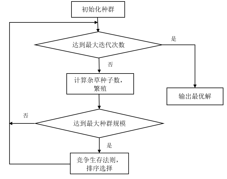
Figure 2 IWO algorithm flow chart
3, MATLAB program implementation
Using the functions provided by MATLAB, the above steps can be easily realized in Matlab environment.
1. Clear environment variables
Before the program runs, clear the variables in Workspace and the commands in Command Window. The specific procedures are as follows:
%% Clear environment variables
clc;
clear;
close all;
2. Problem setting
Before optimization, it is necessary to clarify the objective function of optimization. The specific procedures are as follows:
%% Problem Definition
CostFunction = @(x) Sphere(x);     % objective function
nVar = 5;              % Number of decision variables
VarSize = [1 nVar];    % Decision variable matrix size
VarMin = -10;       % Lower limit of decision variable
VarMax = 10;        % Upper limit of decision variable
The Sphere function code is as follows:
function z = Sphere(x)
%% objective function
    z = sum(x.^2);
end
3. Parameter setting
The code is as follows:
4. Initialize weed population
Before calculation, the weed population needs to be initialized. At the same time, in order to speed up the execution of the program, the storage capacity of some process variables involved in the program needs to be pre allocated. The specific procedures are as follows:
%% Initialization
% Empty plant matrix (including position and fitness values)
empty_plant.Position = [];
empty_plant.Cost = [];
pop = repmat(empty_plant, nPop0, 1);    % Initial population matrix
for i = 1:numel(pop)
    % Initialization location
    pop(i).Position = unifrnd(VarMin, VarMax, VarSize);
    % Initialize fitness value
    pop(i).Cost = CostFunction(pop(i).Position);
end
% Initialize optimal function value history
BestCosts = zeros(MaxIt, 1);
5. Iterative optimization
Iterative optimization is the core of the whole algorithm. Firstly, the standard deviation is calculated according to formula (4), the optimal and worst objective function values are obtained, and the offspring population is initialized; Then the propagation operation is carried out, and the number of seeds produced by each weed individual is calculated according to formula (2); After that, the seeds generated by each weed are traversed, and the seeds generated by the weed obey n (0, σ 2 ) N(0,\sigma^2)N(0, σ 2) And formula (3) generate corresponding individuals and add them to the offspring population; Finally, the parents and children are merged, and the additional members (if redundant) are eliminated according to the competitive survival law to save the optimal solution of each generation.
%% IWO Main Loop
for it = 1:MaxIt
    % Update standard deviation
    sigma = ((MaxIt - it)/(MaxIt - 1))^Exponent * (sigma_initial - sigma_final) + sigma_final;
    % Get the best and worst target values
    Costs = [pop.Cost];
    BestCost = min(Costs);
    WorstCost = max(Costs);
    % Initialize offspring population
    newpop = [];
    % reproduction
    for i = 1:numel(pop)
        % Scale factor
        ratio = (pop(i).Cost - WorstCost)/(BestCost - WorstCost);
        % Number of seeds per weed
        S = floor(Smin + (Smax - Smin)*ratio);
        for j = 1:S
            % Initialize offspring
            newsol = empty_plant;
            % Generate random location
            % randn Is a function that produces a random number or matrix of standard normal distribution
            newsol.Position = pop(i).Position + sigma * randn(VarSize);
            % boundary(lower limit/upper limit)handle
            newsol.Position = max(newsol.Position, VarMin);
            newsol.Position = min(newsol.Position, VarMax);
            % Objective function value of offspring
            newsol.Cost = CostFunction(newsol.Position);
            % Add offspring
            newpop = [newpop
                      newsol];  % #ok
        end
    end
    % Combined population
    pop = [pop
           newpop];
    % Population ranking
    [~, SortOrder] = sort([pop.Cost]);
    pop = pop(SortOrder);
    % Competitive exclusion (remove additional members)
    if numel(pop)>nPop
        pop = pop(1:nPop);
    end
    % Preserve the best population
    BestSol = pop(1);
    % Save optimal function value history
    BestCosts(it) = BestSol.Cost;
    % Show iteration information
    disp(['Iteration ' num2str(it) ': Best Cost = ' num2str(BestCosts(it))]);
end
6. The results show that
In order to observe and analyze the results more intuitively, the results are displayed in the form of graphics. The specific procedures are as follows:
%% Results
figure;
% plot(BestCosts, 'LineWidth', 2);
semilogy(BestCosts, 'r', 'LineWidth', 2);
xlabel('Iteration');
ylabel('Best Cost');
grid on;
The evolution process of IWO algorithm is shown in Figure 3.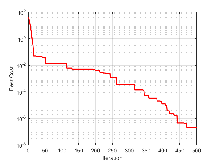
Figure 3 iterative evolution process of Iwo algorithm
Code download https://www.cnblogs.com/matlabxiao/p/14883637.html
4, References
[1] Mehrabian A R , Lucas C . A novel numerical optimization algorithm inspired from weed colonization[J]. Ecological Informatics, 2006, 1(4):355-366.
[2] Kawadia V , Kumar P R . Principles and protocols for power control in wireless ad hoc networks[J]. IEEE Journal on Selected Areas in Communications, 2005, 23(1):76-88.
[3] Meng Fan-zhi, Wang Huan-zhao, He Hui. Connected coverage protocol using cooperative sensing model for wireless sensor networks[J]. Journal of Electronics,2011,39(4):722-799.