1, Background

Giant panda is a national protected animal in China. The survival of giant panda must meet the conditions of certain trough area (exclusive hunting and activity range). Therefore, scientific and accurate analysis of the distribution of pandas is of great significance to reasonably formulate protection measures and evaluate protection effectiveness.

2, Purpose

Through practice, be familiar with the principle and difference of ArcGIS density mapping function, and master how to make a density map meeting the requirements according to the characteristics of deeds sampling data, combined with the density mapping function provided by ArcGIS and other spatial analysis.

3, Request

1) Panda activities have a certain trough range. There is only one or a pair of pandas in a trough range. Assuming that the radius of the panda trough is 5000m, the theoretical maximum trough area is 3.1450005000

2) Although a sampling point represents a panda, different sampling points have different spatial control areas because the survival of pandas has the characteristics of determined slot domain. Assuming that the distribution of panda activity range meets the Tyson polygon centered on the sampling point, how to add this information to the density distribution map is the focus of this exercise.

3) Based on the panda activity footprint data collected in the field, taking the range of each panda trough as the weight, the panda distribution density map in this area is made by using the regional distribution function and density mapping function in ArcGIS.

4, Data

According to the data of panda activity footprints collected in the field, one footprint represents that a panda has been active here, and the same footprint is recorded only once. (\Chp8\Ex3)

5, Calculation principle

Firstly, the area distribution function provided by the grid data spatial analysis module is used to extract the slot area of the panda, and then the theoretical maximum area (assuming a circle with a radius of 5km and an area of 3.141592755 km) is used ²) Divide the extracted panda actual slot area as the weighted value of the sampling point (recorded as the Power field) to generate the panda distribution density map.

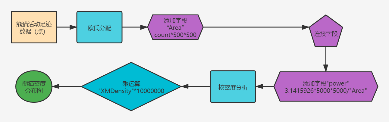
Problem solving ideas:
1) The actual control range of each panda is calculated by European distribution

2) Add the field area to calculate the actual control area of each panda: grid number, grid side length, grid side length

3) Add the power field to calculate the weight: theoretically, the maximum slot area / grid number grid side length grid side length

4) Nuclear density analysis using power field

Operation flow chart:

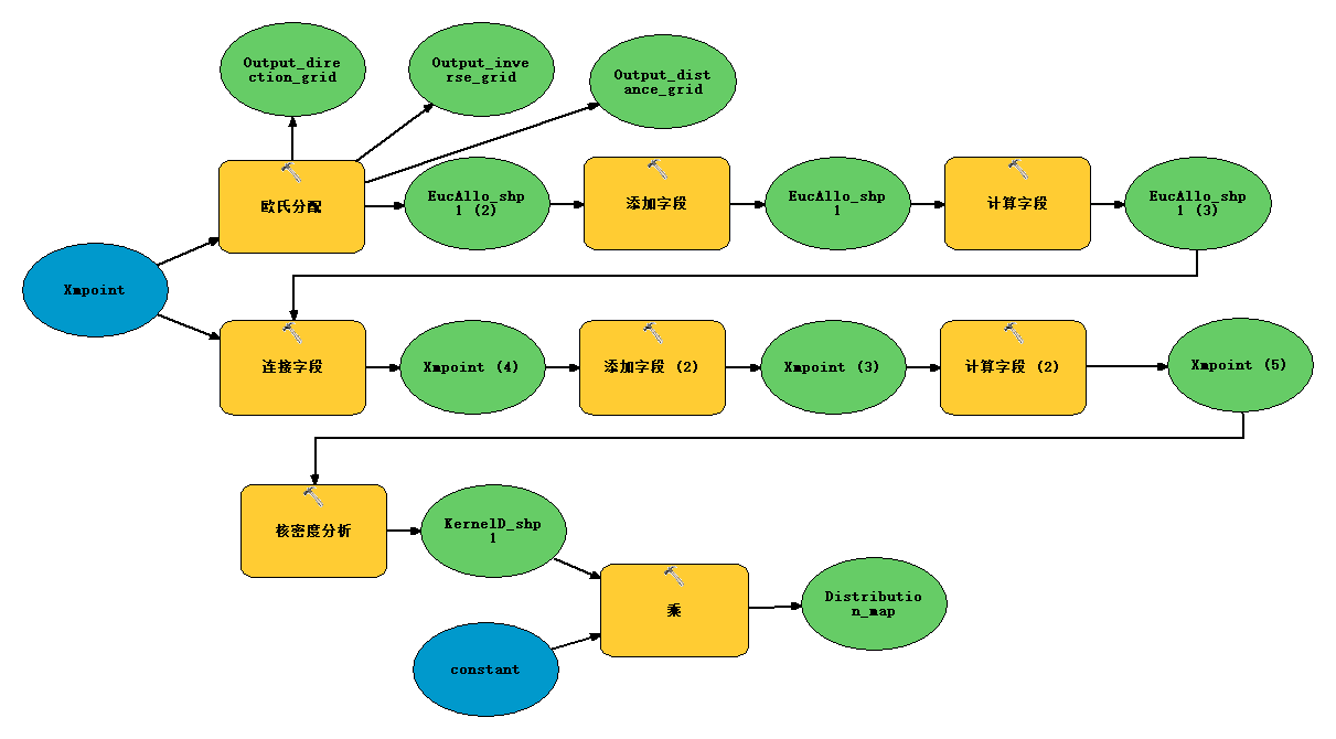
6, Model builder

7, ArcPy implementation

# -*- coding: utf-8 -*-
# ---------------------------------------------------------------------------
# 8-3 panda density map.py
# Created on: 2021-10-10 15:53:34.00000
#   (generated by ArcGIS/ModelBuilder)
# Description: 
# ---------------------------------------------------------------------------

# Import arcpy module
import arcpy
import os


path = raw_input("Please enter the absolute path where the data is located:").decode("utf-8")
paths = path + "\\result"
if not os.path.exists(paths):
    os.mkdir(paths)

# Local variables:
Xmpoint = path + "\\Xmpoint.shp"  # data
Output_distance_grid = "Distance"  # Output the distance grid. The length of the grid base name cannot exceed 13
Output_direction_grid = "Direction"  # Output direction grid, the length of grid basic name cannot exceed 13
Output_inverse_grid = "Inverse"  # Output a reverse grid. The length of the grid base name cannot exceed 13
EucAllo_shp = "EucAllo_shp"  # European distribution output elements
KernelD_shp = "KernelD_shp"  # Output elements of nuclear density analysis
constant = "10000000"
Distribution_map = "Density distribution map"  # The length of the grid base name cannot exceed 13

# Set Geoprocessing environments
print "Set Geoprocessing environments"
arcpy.env.workspace = paths  # working space
arcpy.env.scratchWorkspace = paths  # Temporary workspace
arcpy.env.extent = "15153765.390904 -140950.922884 15227181.528600 -92036.748014"  # Processing range, bottom left and top right

# Process: check whether the fields in the attribute table contain "area" and "power", and delete them if any
fields = arcpy.ListFields(Xmpoint)
for field in fields:
    if fields.name.lower() in ["area", "power"]:
        arcpy.DeleteField_management(Xmpoint, fields.name)

# Process: Euclidean distribution
print "Process: Euclidean distribution"
arcpy.gp.EucAllocation_sa(Xmpoint, EucAllo_shp, "5000", "", "500", "ID", Output_distance_grid, Output_direction_grid, "PLANAR", "", Output_inverse_grid)

# Process: add field
print "Process: Add field"
arcpy.AddField_management(EucAllo_shp, "Area", "LONG", "", "", "", "", "NULLABLE", "NON_REQUIRED", "")

# Process: calculated fields
print "Process: Calculation field"
arcpy.CalculateField_management(EucAllo_shp, "Area", "[COUNT] * 500 *500", "VB", "")

# Process: connection fields
print "Process: Connection field"
arcpy.JoinField_management(Xmpoint, "ID", EucAllo_shp, "Value", "Area")

# Process: add field (2)
print "Process: Add field (2)"
arcpy.AddField_management(Xmpoint, "power", "LONG", "", "", "", "", "NULLABLE", "NON_REQUIRED", "")

# Process: calculated field (2)
print "Process: Calculation field (2)"
arcpy.CalculateField_management(Xmpoint, "power", "3.1415927*5000*5000 / [Area]", "VB", "")

# Process: nuclear density analysis
print "Process: Nuclear density analysis"
arcpy.gp.KernelDensity_sa(Xmpoint, "power", KernelD_shp, "500", "", "SQUARE_MAP_UNITS", "DENSITIES", "PLANAR")

# Process: multiply
print "Process: ride"
arcpy.gp.Times_sa(KernelD_shp, constant, Distribution_map)

rasters = arcpy.ListRasters()
for raster in rasters:
    if u"Distribution map" not in raster:
        print u"Deleting{}".format(raster)
        arcpy.Delete_management(raster)
print "Operation completed~~~"

Pay attention to the notes!

8, Results

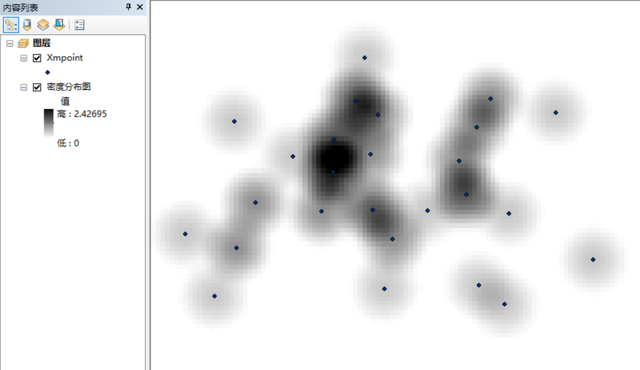
End of experiment byebye~