In financial data analysis or quantitative research, the processing of time series data can not be avoided. Time series refers to the value sequence of a variable measured in time order within a certain time. Common time series data include temperature series that change with time in a day, or stock price series that fluctuate continuously during trading time. Pandas is also widely used in financial data analysis because of its strong time series processing ability. This article introduces the time series processing in pandas. The data used is the market data of Shanghai stock index in 2019.

Time dependent data types

The two most common data types in Pandas timing processing are datetime and timedelta. A datetime can be as shown in the following figure:

As the name suggests, datetime means both date and time, indicating a specific point in time (timestamp). Timedelta indicates the difference between two time points. For example, the timedelta between 2020-01-01 and 2020-01-02 is one day. I believe it is not difficult to understand.

Convert time column to time format

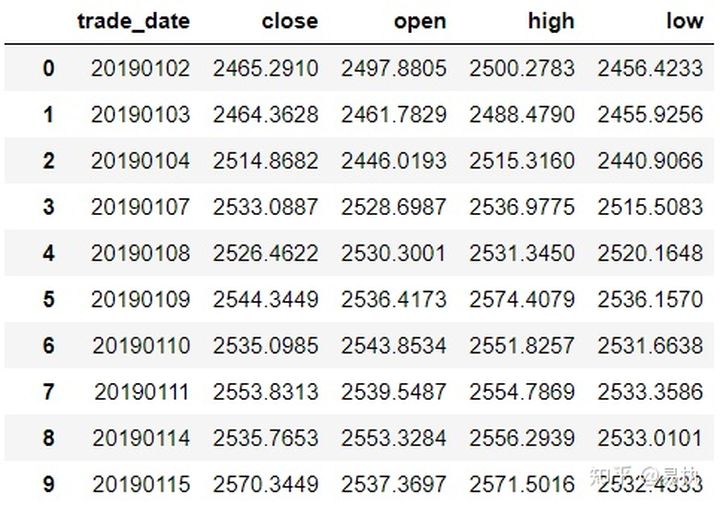
Most of the time, we import data from csv files. At this time, the corresponding time column in Dataframe is in the form of string, as follows:

In [5]: data.trade_date.head()
Out[5]:
0    20190102
1    20190103
2    20190104
3    20190107
4    20190108
Name: trade_date, dtype: object

Using pd.to_datetime(), which can convert the corresponding column to datetime64 in Pandas for later processing

In [11]: data["trade_date"] = pd.to_datetime(data.trade_date)

In [12]: data.trade_date.head()
Out[12]:
0   2019-01-02
1   2019-01-03
2   2019-01-04
3   2019-01-07
4   2019-01-08
Name: trade_date, dtype: datetime64[ns]

Index of time series

The index in time series is similar to the ordinary index in Pandas. Most of the time, you call. loc[index,columns] to index the corresponding index. Go directly to the code

In [20]: data1 = data.set_index("trade_date")

# June 2019 data
In [21]: data1.loc["2019-06"].head()
Out[21]:
                close       open       high        low
trade_date
2019-06-03  2890.0809  2901.7424  2920.8292  2875.9019
2019-06-04  2862.2803  2887.6405  2888.3861  2851.9728
2019-06-05  2861.4181  2882.9369  2888.7676  2858.5719
2019-06-06  2827.7978  2862.3327  2862.3327  2822.1853
2019-06-10  2852.1302  2833.0145  2861.1310  2824.3554

# Data from June 2019 to August 2019
In [22]: data1.loc["2019-06":"2019-08"].tail()
Out[22]:
                close       open       high        low
trade_date
2019-08-26  2863.5673  2851.0158  2870.4939  2849.2381
2019-08-27  2902.1932  2879.5154  2919.6444  2879.4060
2019-08-28  2893.7564  2901.6267  2905.4354  2887.0115
2019-08-29  2890.9192  2895.9991  2898.6046  2878.5878
2019-08-30  2886.2365  2907.3825  2914.5767  2874.1028

Extract time / date attributes

In the process of time series data processing, the following requirements often need to be realized:

• Find the number of weeks corresponding to a date (2019-06-05 is the week)
• Judge the day of the week (2020-01-01 is the day of the week)
• Judge which quarter a date is (which quarter 2019-07-08 belongs to)

......

When the time column in the data (trade_date column in this data) has been converted to datetime64 format, you can quickly obtain the desired result by calling the. dt interface. The following table lists the common attributes provided by the. dt interface:

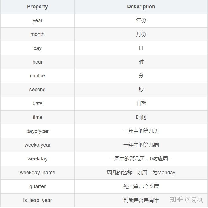
Specific demonstration (only 2019-01-02 information is shown below):

# What day of the year
In [13]: data.trade_date.dt.dayofweek[0]
Out[13]: 2

# Return corresponding date
In [14]: data.trade_date.dt.date[0]
Out[14]: datetime.date(2019, 1, 2)

# Return weeks
In [15]: data.trade_date.dt.weekofyear[0]
Out[15]: 1

# Return day of week
In [16]: data.trade_date.dt.weekday_name[0]
Out[16]: 'Wednesday'

resample

resample translates to resampling, which is described in the official documents

resample() is a  time-based groupby

In my opinion, this is the most important function in Pandas time series processing, and it is also the top priority of this paper.

According to whether the sampling is from low frequency to high frequency or from high frequency to low frequency, it can be divided into up sampling and down sampling. Let's see what down sampling is first

• Downsampling

As an example, the data we use is the daily level data of Shanghai stock index in 2019. What should we do if we want to find the average closing price of each quarter now?

Calculating quarterly level data from daily level data is an aggregation operation from high frequency to low frequency. In fact, it is similar to group by operating quarterly. It is written in resample

In [32]: data.resample('Q',on='trade_date')["close"].mean()
Out[32]:
trade_date
2019-03-31    2792.941622
2019-06-30    3010.354672
2019-09-30    2923.136748
2019-12-31    2946.752270
Freq: Q-DEC, Name: close, dtype: float64

Where 'Q' is sampled quarterly, and on specifies the datetime column (if the index is Datetimeindex, on does not need to specify, and downsampling is performed according to the index by default). The whole process is illustrated as follows:

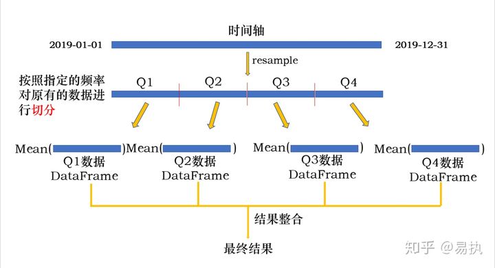
The whole process is actually a group by process:

• The original data is divided into different group s according to the specified frequency
• Perform operations on different group s
• Integrate operation results

Among them, the frequency of segmentation can be any time frequency, quarterly Q, monthly M, week W, N day ND, or H and T. of course, if the frequency after segmentation is less than the original time frequency, it is the upsampling we will talk about below.

• Liter sampling

When the sampling frequency is lower than the original frequency, it is called ascending sampling. Upsampling is a more fine-grained division of the original time granularity, so missing values will be generated during upsampling. Next, take the data from 2019-01-02 to 2019-01-03 and demonstrate it according to the frequency of 6H:

In [24]: example
Out[24]:
                close
trade_date
2019-01-02  2465.2910
2019-01-03  2464.3628

In [25]: example.resample('6H').asfreq()
Out[25]:
                         close
trade_date
2019-01-02 00:00:00  2465.2910
2019-01-02 06:00:00        NaN
2019-01-02 12:00:00        NaN
2019-01-02 18:00:00        NaN
2019-01-03 00:00:00  2464.3628

Applying. asfreq() to the result after resample will return the result under the new frequency. You can see that the missing value is generated after the upsampling. If you want to fill in missing values, you can fill in. bfill() backward or. Fill() forward:

# Fill forward. The missing value is 2465.2910
In [29]: example.resample('6H').ffill()
Out[29]:
                         close
trade_date
2019-01-02 00:00:00  2465.2910
2019-01-02 06:00:00  2465.2910
2019-01-02 12:00:00  2465.2910
2019-01-02 18:00:00  2465.2910
2019-01-03 00:00:00  2464.3628

# Fill backward. The missing value is 2464.3628
In [30]: example.resample('6H').bfill()
Out[30]:
                         close
trade_date
2019-01-02 00:00:00  2465.2910
2019-01-02 06:00:00  2464.3628
2019-01-02 12:00:00  2464.3628
2019-01-02 18:00:00  2464.3628
2019-01-03 00:00:00  2464.3628

To sum up, resample can sample any frequency freq of the original time series. If it is up sampling from low frequency to high frequency, it is down sampling from high frequency to low frequency. The whole operation process is basically the same as that of groupby, so you can also apply and transform the object after resample. The specific operation and principle will not be explained here. It can be compared with groupby. See this article Pandas data analysis -- a detailed explanation of Groupby.