Hello, I'm Pippi. In fact, the volume of this pandas tutorial is very serious. Cai Ge, Xiao P and others have written a lot of articles. This article is contributed by fans [ancient moon and stars]. They have sorted out some basic materials in their own learning process, sorted them out and written them, and sent them here for everyone to study together.

Getting started with Pandas

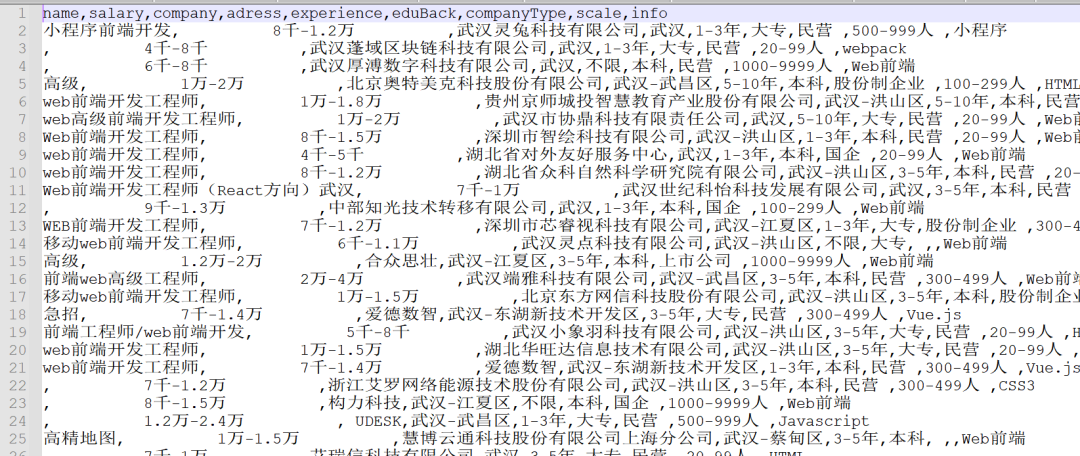
This paper mainly introduces various basic operations of pandas in detail. The source file is zljob CSV, which can be obtained privately. The following figure is a list of the original data.

pandas official website:

https://pandas.pydata.org/pandas-docs/stable/getting_started/index.html

Directory structure:

• Generate data table
• Basic operation of data sheet
• Data cleaning
• time series

I Generate data table

1.1 data reading

Generally, most of the data types we get are csv or excel files. Only csv is given here,

• Read csv file

pd.read_csv()

• Read excel file

pd.read_excel()

1.2 creation of data

pandas can create two data types, series and DataFrame;

• Create a series (similar to a list, which is a one-dimensional sequence)

• s = pd.Series([1,2,3,4,5])

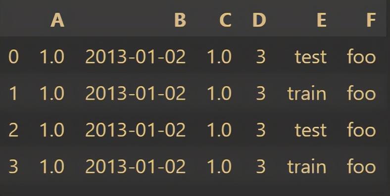
• Create dataframe (similar to excel table, which is two-dimensional data)

• df2 = pd.DataFrame(
  { "A": 1.0,
  "B": pd.Timestamp("20130102"),
  "C": pd.Series(1, index=list(range(4)), dtype="float32"),
  "D": np.array([3] * 4, dtype="int32"),
  "E": pd.Categorical(["test", "train", "test", "train"]),
  "F": "foo",
  })

2, Basic operation of data table

2.1 data viewing

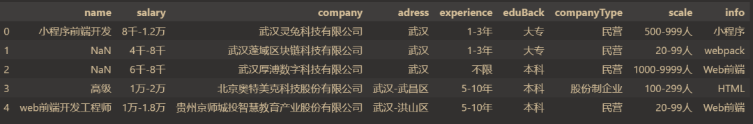
• View the first five lines
• data. The head() # head() parameter indicates the first few lines, and the default value is 5

• essential information

data.shape

(990, 9)

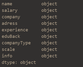
data.dtypes

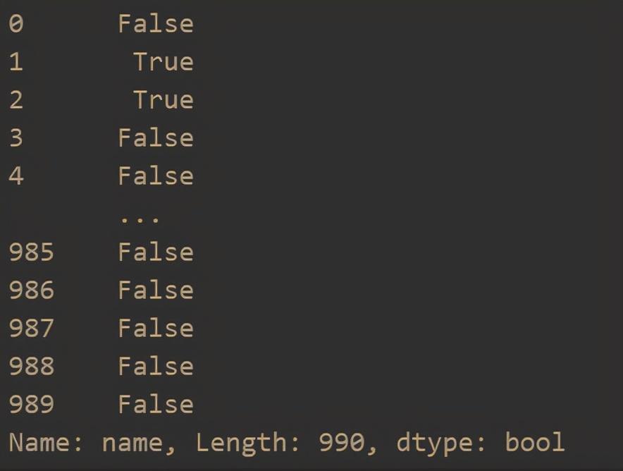
• View null values

data['name'].isnull() # Check whether the name column has a null value

2.2 operation of rows and columns

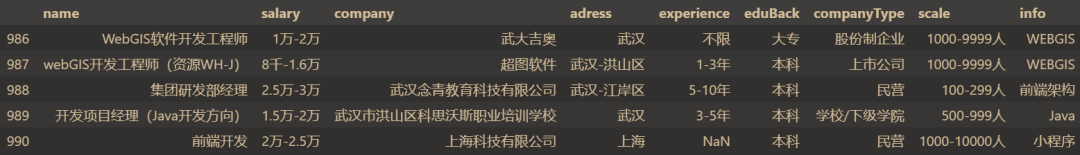
• Add a column

dic = {'name':'Front end development','salary':2 ten thousand-2.5 ten thousand,  'company':'Shanghai Technology Co., Ltd',  'adress':'Shanghai','eduBack':'undergraduate','companyType':'privately operated',  'scale':1000-10000 people,'info':'Applet'}

df = pd.Series(dic)

df.name = 38738

data = data.append(df)

data.tail()

result:

• Delete a row

data = data.drop([990])

• Add a column

data  = data["xx"] = range(len(data))

• Delete a column

data = data.drop('Serial number',axis=1)

Axis stands for axial direction, axis=1 stands for vertical direction (delete a column)

2.3 index operation

• loc
• loc is mainly based on labels, including row labels (index) and column labels (columns), that is, row names and column names. DF can be used loc [index_name, col_name], select the data at the specified location. Other uses are:
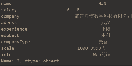
• 1. Use a single label data loc[10,'salary']

  90000-13000.22 list of individual tags

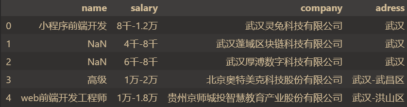
  data.loc[:,'name'][:5]
  3. Slice object data of label loc[:,['name','salary']][:5]
• iloc

iloc is a location-based index, which is selected by using the index sequence number of the element on each axis. If the sequence number exceeds the range, an IndexError will be generated. When slicing, the sequence number is allowed to exceed the range. The usage includes:

1. Use integer

data.iloc[2] # Take out the row with index 2

2. Use list or array

data.iloc[:5]

3. Slice object

data.iloc[:5,:4] # Split by, slice 5 rows in the front and 4 columns in the back

The common methods are shown above.

2.4 hierarchical index

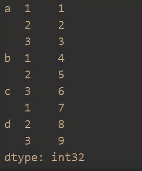
• series hierarchical index

s = pd.Series(np.arange(1,10),index=[list('aaabbccdd'),[1,2,3,1,2,3,1,2,3]])

• dataframe hierarchical index

df = pd.DataFrame(np.arange(12).reshape(4,3),index=[['a','a','b','b'],[1,2,1,2]],columns=[['X','X','Y'],['m','n','t']])

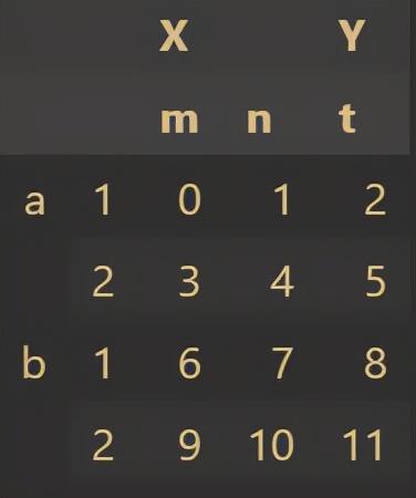
Hierarchical index is applied to analyze multiple features when there are many eigenvalues of target data.

3, Data preprocessing

3.1 missing value handling

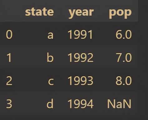
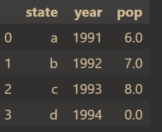
First create a simple table:

df = pd.DataFrame({'state':['a','b','c','d'],'year':[1991,1992,1993,1994],'pop':[6.0,7.0,8.0,np.NaN]})

df

The results are as follows:

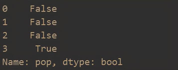
Judge missing value

df['pop'].isnull()

The results are as follows:

Fill in missing values

df['pop'].fillna(0,inplace=True) # Fill missing values with 0

df

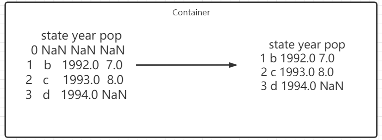
Delete missing values

data.dropna(how = 'all')    # When this parameter is passed in, only those rows with all missing values will be discarded 

The results are as follows:

Of course, there are other situations:

data.dropna(axis = 1)       # Discard columns with missing values (this is not usually done, which will delete a feature)

data.dropna(axis=1,how="all")   # Discard those columns that are all missing values

data.dropna(axis=0,subset = ["Age", "Sex"])   # Discard rows with missing values in the 'Age' and 'Sex' columns

We will not show them one by one here (the principle is the same)

3.2 character processing

• Clear character spaces

df['A']=df['A'].map(str.stri())

• toggle case

df['A'] = df['A'].str.lower()

3.3 repeated value processing

• Delete duplicate values that appear later

df['A'] = df['A'].drop_duplicates() # Duplicate data after a column is cleared

• Delete the first duplicate value

df['A'] = df['A'].drop_duplicates(keep=last) # # Duplicate data in a column is cleared

• Data replacement

df['A'].replace('sh','shanghai') # Same as string substitution

4, Data table operation

grouping

groupby

group = data.groupby(data['name']) # Group by position name

group

Group by position name:

<pandas.core.groupby.generic.DataFrameGroupBy object at 0x00000265DBD335F8>

When we get an object, we can calculate the average value and sum;

Of course, there is no basis for grouping multiple problems;

polymerization

concat():

pd.concat(

    objs,

    axis=0,

    join="outer",

    ignore_index=False,

    keys=None,

    levels=None,

    names=None,

    verify_integrity=False,

    copy=True, 

)

The parameters on the official website are explained as follows:

• Objs: sequence or mapping of series or DataFrame objects. If dict is passed, the sorted key will be used as the keys parameter, unless passed, in which case the value will be selected (see below). Any None objects will be silently deleted unless they are all None, in which case ValueError will be raised.
• Axis: {0, 1,...}, the default is 0. The axis along which to connect.
• Join: {inner ','outer'}, the default is' outer '. How to handle indexes on other axes. The exterior is used for union and the interior is used for intersection.
• ignore_index: Boolean value. The default value is False. If True, do not use index values on the tandem axis. The resulting axis will be marked 0,..., n - 1. This is useful if you connect objects without meaningful index information on the connection axis. Note that index values on other axes are still valid in the connection.
• keys: sequence, none by default. Use the passed key as the outermost layer to build a hierarchical index. If multiple levels are passed, tuples should be included.
• levels: sequence list, none by default. The specific level (one value only) used to build the MultiIndex. Otherwise, they will be inferred from the key.
• names: list, none by default. The name of the level in the generated hierarchical index.
• verify_integrity: Boolean value. The default value is False. Check that the new tandem axis contains duplicates. Compared with the actual data concatenation, this can be very expensive.
• Copy: Boolean value. The default value is true. If False, do not copy data unnecessarily.

Test:

df1 = pd.DataFrame(

    {

        "A": ["A0", "A1", "A2", "A3"],

        "B": ["B0", "B1", "B2", "B3"],

        "C": ["C0", "C1", "C2", "C3"],

        "D": ["D0", "D1", "D2", "D3"],

    },

    index=[0, 1, 2, 3],

)

df2 = pd.DataFrame(

    {

        "A": ["A4", "A5", "A6", "A7"],

        "B": ["B4", "B5", "B6", "B7"],

        "C": ["C4", "C5", "C6", "C7"],

        "D": ["D4", "D5", "D6", "D7"],

    },

    index=[4, 5, 6, 7],

)

df3 = pd.DataFrame(

    {

        "A": ["A8", "A9", "A10", "A11"],

        "B": ["B8", "B9", "B10", "B11"],

        "C": ["C8", "C9", "C10", "C11"],

        "D": ["D8", "D9", "D10", "D11"],

    },

    index=[8, 9, 10, 11],

)

frames = [df1, df2, df3]

result = pd.concat(frames)

result

The results are as follows:

merge()

pd.merge(

    left,

    right,

    how="inner",

    on=None,

    left_on=None,

    right_on=None,

    left_index=False,

    right_index=False,

    sort=True,

    suffixes=("_x", "_y"),

    copy=True,

    indicator=False,

    validate=None,

)

Common parameter explanations are given here:

• left: a DataFrame or named Series object; right: another DataFrame or named Series object;
• on: name of the column or index level to be added;
• left_on: the column or index level of the left DataFrame or Series is used as the key. It can be column name, index level name or array with length equal to DataFrame or Series; right_on: the column or index level from the correct DataFrame or Series is used as the key. It can be a column name, an index level name, or an array with a length equal to the length of DataFrame or Series
• left_index: if True, use the index (row label) in the DataFrame or Series on the left as its connection key; right_index: and left_index is the same as the correct DataFrame or Series;
• how: 'left', 'right', 'outer', one of 'inner'. The default is inner For a more detailed description of each method, see below.

Test:

left = pd.DataFrame(

    {

        "key": ["K0", "K1", "K2", "K3"],

        "A": ["A0", "A1", "A2", "A3"],

        "B": ["B0", "B1", "B2", "B3"],

    }

)

right = pd.DataFrame(

    {

        "key": ["K0", "K1", "K2", "K3"],

        "C": ["C0", "C1", "C2", "C3"],

        "D": ["D0", "D1", "D2", "D3"],

    }

)

result = pd.merge(left, right, on="key")

result

The results are as follows:

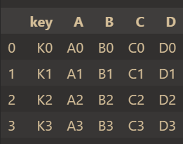
The same field is' key ', so specify on='key' to merge.

5, Time series

5.1 generate a time range

date = pd.period_range(start='20210913',end='20210919')

date

Output result:

PeriodIndex(['2021-09-13', '2021-09-14', '2021-09-15', '2021-09-16', '2021-09-17', '2021-09-18', '2021-09-19'], dtype='period[D]', freq='D')

5.2 application of time series in pandas

index = pd.period_range(start='20210913',end='20210918')

df = pd.DataFrame(np.arange(24).reshape((6,4)),index=index)

df

Output result:

6, Summary

This article is based on the source file zljob CSV, which performs some pandas operations and demonstrates the common data processing operations of pandas library. Due to the complex functions of pandas, please refer to the official website for details