In daily data analysis, it is often necessary to divide the data into different groups according to a certain (multiple) field for analysis. For example, in the field of e-commerce, the total sales of the country are divided according to provinces, and the changes of sales in provinces are analyzed. In the field of social networking, users are subdivided according to portraits (gender and age) to study users' use and preferences. In Pandas, the above data processing operations are mainly completed by groupby. This article introduces the basic principle of groupby and the corresponding agg, transform and apply operations.

For the convenience of subsequent diagrams, 10 sample data generated by simulation are adopted. The codes and data are as follows:

company=["A","B","C"]
​
data=pd.DataFrame({
    "company":[company[x] for x in np.random.randint(0,len(company),10)],
    "salary":np.random.randint(5,50,10),
    "age":np.random.randint(15,50,10)
}
)

1, Basic principles of Groupby

In pandas, the code to realize grouping operation is very simple. Only one line of code is needed. Here, the above data sets are divided according to the company field:

In [5]: group = data.groupby("company")

After inputting the above code into ipython, you will get a DataFrameGroupBy object

In [6]: group
Out[6]: <pandas.core.groupby.generic.DataFrameGroupBy object at 0x000002B7E2650240>

What is the generated DataFrameGroupBy? What happens after data is groupby? The result returned by ipython is its memory address, which is not conducive to intuitive understanding. In order to see what is inside the group, here we convert the group into a list:

In [8]: list(group)
Out[8]:
[('A',   company  salary  age
  3       A      20   22
  6       A      23   33), 
 ('B',   company  salary  age
  4       B      10   17
  5       B      21   40
  8       B       8   30), 
 ('C',   company  salary  age
  0       C      43   35
  1       C      17   25
  2       C       8   30
  7       C      49   19)]

After converting to the form of list, you can see that the list is composed of three tuples. In each tuple, the first element is a group (grouped by company, so it is finally divided into a, B and C), and the second element is the DataFrame under the corresponding group. The whole process can be illustrated as follows:

To sum up, the process of groupby is to divide the original DataFrame into several grouped dataframes according to the field of groupby (here is company), and there are as many grouped dataframes as there are groups. Therefore, a series of operations after groupby (such as agg, apply, etc.) are based on sub DataFrame operations. After understanding this, we can basically understand the main principle of groupby operation in Pandas. Let's talk about the common operations after groupby.

2, agg aggregation operation

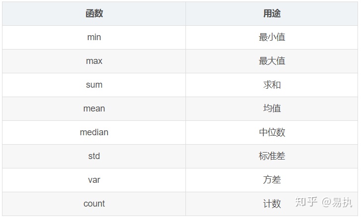
Aggregation is a very common operation after groupby. Friends who can write SQL should be very familiar with it. Aggregation operations can be used to sum, mean, maximum, minimum, etc. the following table lists the common aggregation operations in Pandas.

For the sample dataset, if I want to find the average age and average salary of employees in different companies, I can follow the following code:

In [12]: data.groupby("company").agg('mean')
Out[12]:
         salary    age
company
A         21.50  27.50
B         13.00  29.00
C         29.25  27.25

If you want to find different values for different columns, such as calculating the average age and median salary of employees in different companies, you can use the dictionary to specify the aggregation operation:

In [17]: data.groupby('company').agg({'salary':'median','age':'mean'})
Out[17]:
         salary    age
company
A          21.5  27.50
B          10.0  29.00
C          30.0  27.25

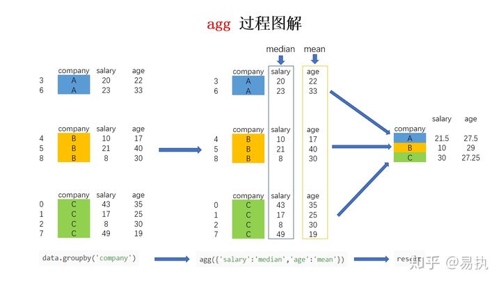
The agg polymerization process can be illustrated as follows (the second example is taken as an example):

3, transform

What kind of data operation is transform? What's the difference between and agg? In order to better understand the difference between transform and agg, the following is a comparison from the actual application scenario.

In the above agg, we learned how to calculate the average salary of employees in different companies. If we need to add a new column of AVG in the original data set now_ Salary, which represents the average salary of the company in which the employee works (employees of the same company have the same average salary), how to achieve it? If you calculate according to the normal steps, you need to first obtain the average salary of different companies, and then fill in the corresponding position according to the corresponding relationship between employees and companies. Without transform, the implementation code is as follows:

In [21]: avg_salary_dict = data.groupby('company')['salary'].mean().to_dict()
​
In [22]: data['avg_salary'] = data['company'].map(avg_salary_dict)
​
In [23]: data
Out[23]:
  company  salary  age  avg_salary
0       C      43   35       29.25
1       C      17   25       29.25
2       C       8   30       29.25
3       A      20   22       21.50
4       B      10   17       13.00
5       B      21   40       13.00
6       A      23   33       21.50
7       C      49   19       29.25
8       B       8   30       13.00

If you use transform, you only need one line of code:

In [24]: data['avg_salary'] = data.groupby('company')['salary'].transform('mean')
​
In [25]: data
Out[25]:
  company  salary  age  avg_salary
0       C      43   35       29.25
1       C      17   25       29.25
2       C       8   30       29.25
3       A      20   22       21.50
4       B      10   17       13.00
5       B      21   40       13.00
6       A      23   33       21.50
7       C      49   19       29.25
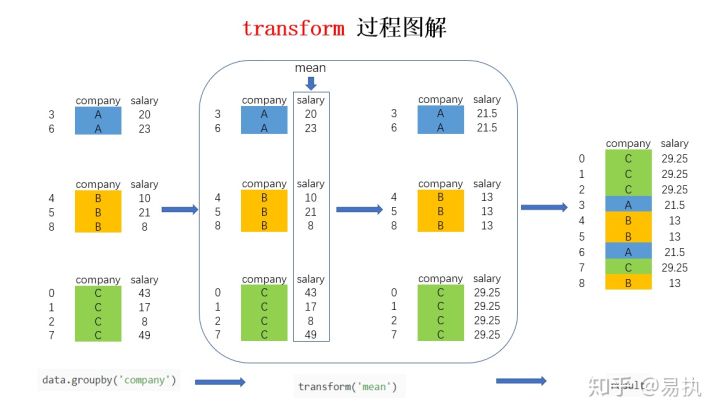
8       B       8   30       13.00

Let's take a graphical look at the implementation process of transform after groupby (for a more intuitive display, the company column is added in the figure. In fact, according to the above code, there is only the salary column):

The big box in the figure shows the difference between transform and agg. For agg, the accounting calculates the corresponding mean values of companies A, B and C and returns them directly. However, for transform, the corresponding results will be obtained for each piece of data. The samples in the same group will have the same values. After calculating the mean values in the group, the results will be returned in the order of the original index, If you don't understand, you can compare this picture with agg that one.

4, apply

apply should be an old friend of everyone. It is more flexible than agg and transform. It can pass in any custom function to realize complex data operation. stay Pandas data processing three board axe -- detailed explanation of map, apply and applymap In, the use of apply is introduced. What is the difference between using apply after groupby and the previous introduction?

There are differences, but the whole implementation principle is basically the same. The difference between the two is that for the application after groupby, the basic operation unit is DataFrame, and the basic operation unit of the application described earlier is Series. Let's take a case to introduce the use of apply after groupby.

Suppose I need to obtain the data of the oldest employees in each company, how can I achieve it? It can be implemented with the following code:

In [38]: def get_oldest_staff(x):
    ...:     df = x.sort_values(by = 'age',ascending=True)
    ...:     return df.iloc[-1,:]
    ...:
​
In [39]: oldest_staff = data.groupby('company',as_index=False).apply(get_oldest_staff)
​
In [40]: oldest_staff
Out[40]:
  company  salary  age  
0       A      23   33       
1       B      21   40       
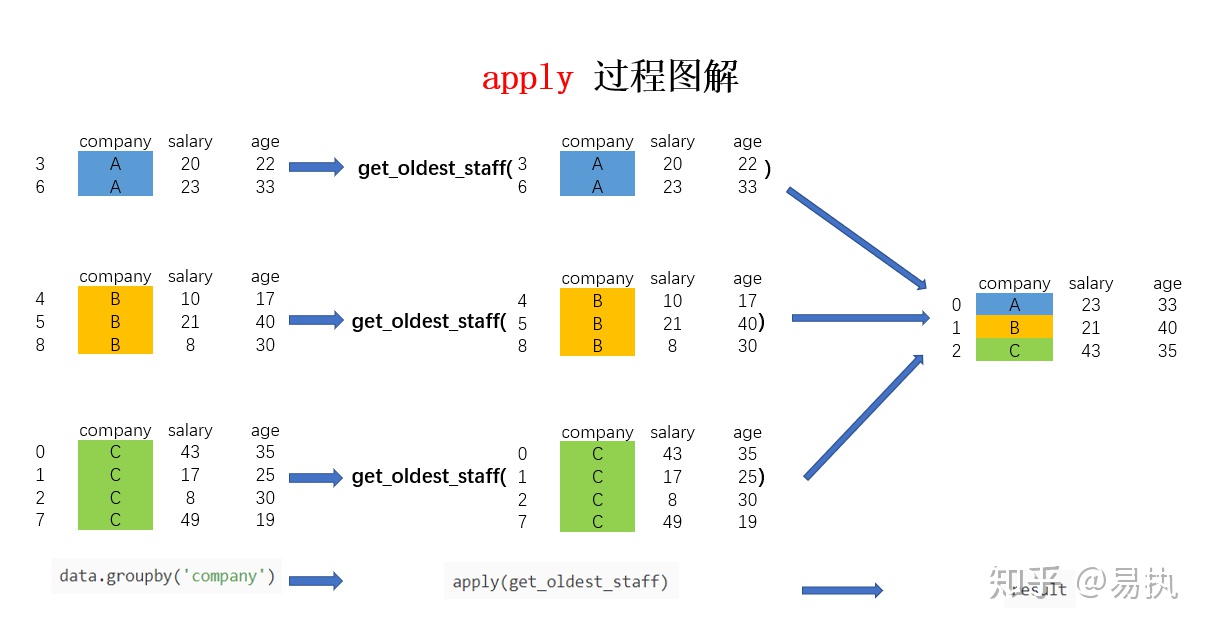
2       C      43   35      

In this way, the data of the oldest employees in each company are obtained. The whole process is illustrated as follows:

You can see that the principle of application here is basically the same as that described in the previous article, except that the parameters of the incoming function change from Series to the grouped DataFrame here.

Finally, here's a little suggestion about the use of apple. Although Apple has greater flexibility, the operation efficiency of Apple will be slower than agg and transform. Therefore, for the problems that groupby can solve with agg and transform in the future, it is better to use these two methods. If it can't be solved, it is considered to use apply for operation.