preface

Original paper address: https://arxiv.org/abs/1905.11946.

This blog has references:

Sunflower mung bean: EfficientNet network explanation.

bilibili: Building EfficientNet network with pytoch.

1, Background

\quad Since the proposal of Alex net network in 2012, convolutional neural network has been developed in the field of computer vision for 9 years. In this process, many network models have been proposed successively, lenet - > AlexNet - > VGg - > googlenet - > RESNET - > senet... These networks have one thing in common, that is, they are all manually designed networks. When reproducing these network codes, you may often have these questions: why should the input image resolution of the network be fixed to 224x224? Why should the number of convolutions be set to this value? Why is the depth of the network so large? If you want to ask the designer these questions, the reply is estimated to be four words - engineering experience. Really can only rely on experience? Really can only rely on Metaphysics? Of course not, so this paper is to explore the impact of the depth, width and resolution of the input image on the network and how they are related.

2, Thesis thought

2.1 theoretical and experimental

\quad In previous papers, one of the width, depth and resolution of the input image is usually adjusted for manual tuning. Some will increase the width in the baseline network as shown in figure (a), that is, increase or decrease the number of volume cores (increase the channel of feature map) to improve the performance of the network, as shown in figure (b); Some will add depth to the baseline network, as shown in figure (a), that is, use more layer structures to improve the performance of the network, as shown in figure (a) © As shown in; Some will increase the resolution of the input picture in the baseline network as shown in figure (a) to improve the performance of the network, as shown in figure (d); However, we all know that depth, width and resolution can never be independent of each other, but depend on each other. Therefore, in this paper, the network width, depth and resolution of the input network will be added to improve the network performance, as shown in figure (e):

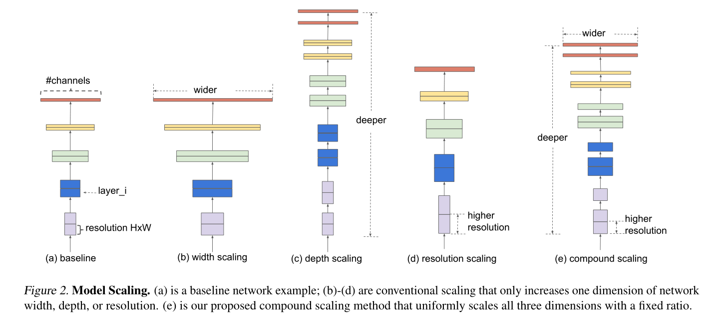
• According to the previous intuitive experience, increasing the depth of the network can get a richer and more complex feature map, and can be well applied to other tasks. However, if the depth of the network is too deep, it will face the problems of gradient disappearance and difficult training.
  The intuition is that deeper ConvNet can capture richer and more complex features, and generalize well on new tasks. However, deeper networks are also more difficult to train due to the vanishing gradient problem
• Increasing the width of the network can obtain higher fine-grained features and easier to train, but it is often difficult to learn deeper features for networks with large width and shallow depth.
  wider networks tend to be able to capture more fine-grained features and are easier to train. However, extremely wide but shallow networks tend to have difficulties in capturing higher level features.
• Increasing the image resolution of the input network can potentially obtain higher fine-grained feature templates, but for very high input resolution, the gain of accuracy will also be reduced. And large resolution images will increase the amount of calculation.
  With higher resolution input images, ConvNets can potentially capture more fine-grained patterns. but the accuracy gain diminishes for very high resolutions.

\quad The following figure shows the statistical results obtained by adding Width, Depth and resolution to the baseline (efficient netb-0). It can be seen that when adding a single element, the Accuracy will end when it increases to about 80%.

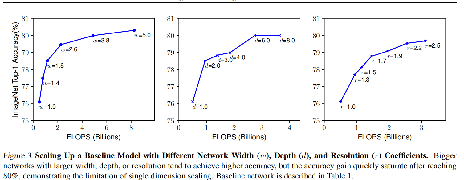
Conclusion 1. Any dimension of scaling width, depth and resolution of input image can increase accuracy, but it will tend to be stable to a certain extent.

\quad Then the author did another experiment, as shown in the figure below, using different combinations of d and r, and then constantly changing the width of the network to obtain four curves as shown in the figure below. Through analysis, it can be found that under the same FLOPs, the effect of increasing d and r at the same time is the best. (blue means depth and resolution remain unchanged and width changes; green means resolution remains unchanged, d e p t h = 2 ∗ d e p t h depth=2*depth Change the width when depth=2 * depth; Yellow means depth remains unchanged, r e s o l u t i o n = 1.3 ∗ r e s o l u t i o n resolution=1.3*resolution resolution=1.3 * change the width in the case of resolution; Red indicates d e p t h = 2 ∗ d e p t h depth=2*depth depth=2∗depth， r e s o l u t i o n = 1.3 ∗ r e s o l u t i o n resolution=1.3*resolution resolution=1.3 * change width in the case of resolution)

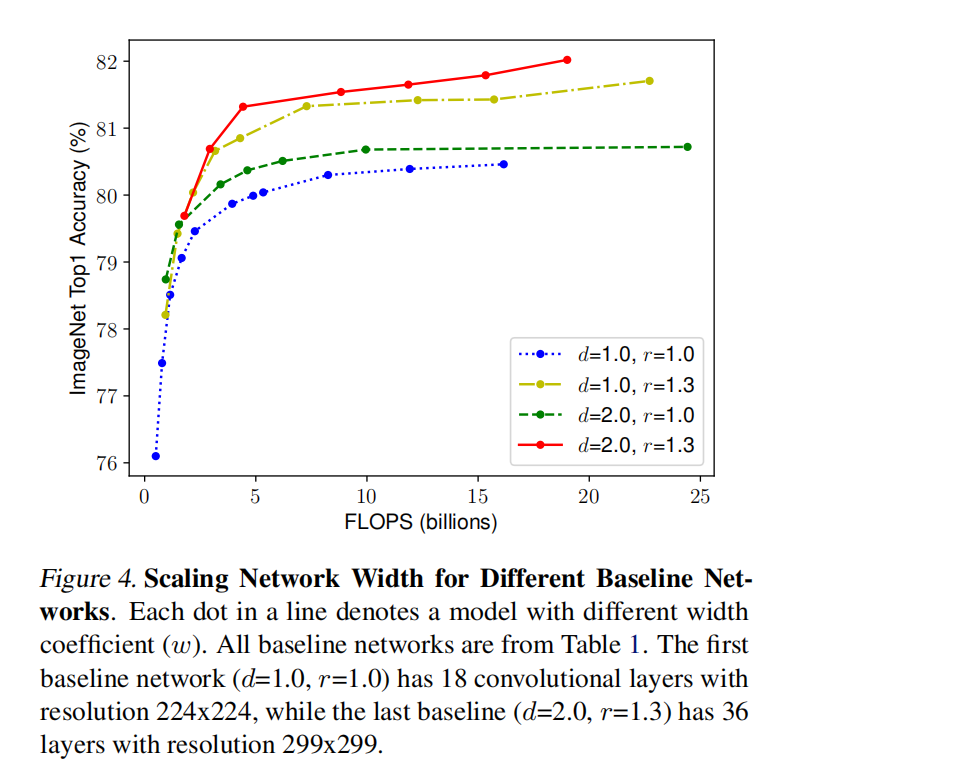
Conclusion 2. It is very important to balance these three dimensions in the process of scaling width, depth and resolution of input image.

2.2 further formula discussion

In order to explore this problem, the author first abstracts the whole network:
N ( d , w , r ) = ⨀ i = 1 ... s F i L i ( X ⟨ H i , W i , C i ⟩ ) N(d, w, r)= \underset{i=1...s}{\bigodot} F^{Li}_i(X_{\langle H_i,W_i,C_i\rangle}) N(d,w,r)=i=1...s⨀​FiLi​(X⟨Hi​,Wi​,Ci​⟩​)

Of which:

• ⨀ i = 1 ... s \underset{i=1...s}{\bigodot} i=1... s ⨀ indicates continuous multiplication
• F i F_i Fi indicates an operation, F i L i F^{Li}_i FiLi said F i F_i Fi operation in S t a g e i Stage_i Number of executions in Stagei #, L i Li Li is the number of executions and depth
• X indicates input S t a g e i Stage_i Input tensor of Stagei. ⟨ H i , W i , C i ⟩ {\langle H_i,W_i,C_i\rangle} ⟨ Hi, Wi, Ci ⟩ indicates the height, width (resolution) and Channels(width) of X

To explore d , w , r d, w, r d. The influence of the three factors W and R on the final accuracy will be d , w , r d, w, r d. When w and R are added to the formula, we can get the abstract optimization problem (under the specified resource constraints), where s . t . s.t. s.t. representative restrictions:

Of which:

• d d d is used to scale the depth L i ^ \widehat{L_i} Li​ ​
• r r r is used to scale the resolution, i.e. influence H i ^ \widehat{H_i} Hi​ And $\ widehat{W_i}
• w w w is used to scale the channel of the characteristic matrix, that is, the influence C i ^ \widehat{C_i} Ci​ ​
• target_memory is a memory limit
• target_flops is the FLOPs limit

As mentioned earlier, the three dimensions of network depth, width and input resolution are not independent of each other. They are interdependent. Therefore, exploring the relationship between d, w and r is actually very complex. Then, the author proposes a new compound model scaling method.

The author's idea is that all convolution layers of a convolution network must be uniformly extended through the same proportional constant. This sentence means that three parameters are multiplied by Changshu magnification. Therefore, a model expansion problem is described in mathematical language as:

be careful:

• FLOPs calculation method of a layer: f e a t u r e w feature_w featurew​ x f e a t u r e h feature_h featureh​ x f e a t u r e c feature_c featurec​ x k e r n e l w kernel_w kernelw​ x k e r n e l h kernel_h kernelh​ x k e r n e l n u m b e r kernel_{number} kernelnumber​
• The relationship between FLOPs and depth is: when depth is doubled, FLOPs is doubled
• The relationship between FLOPs and width is that when the width is doubled (i.e. the channel is doubled), FLOPs will be doubled by four times. When the width is doubled, the number of channels or convolution kernels of the input characteristic matrix and the output characteristic matrix will be doubled, so the FLOPs will be doubled by four times
• The relationship between FLOPs (theoretical calculation) and resolution is that when the resolution is doubled, FLOPs will also be quadrupled, which is similar to the above, because the width and height of the characteristic matrix will be doubled.

Therefore, the total FLOPs magnification can be approximated ( α . β 2 . γ 2 ) (\alpha . \beta^2 . \gamma^2) ( α.β two γ 2) To indicate when the limit α . β 2 . γ 2 ≈ 2 \alpha . \beta^2 . \gamma^2\approx2 α.β two γ When 2 ≈ 2, for any ϕ \phi ϕ In general, FLOPs have increased considerably 2 ϕ 2^\phi two ϕ Times.

3, EfficientNet-v1 network structure

Network structure of EfficientNet-B0

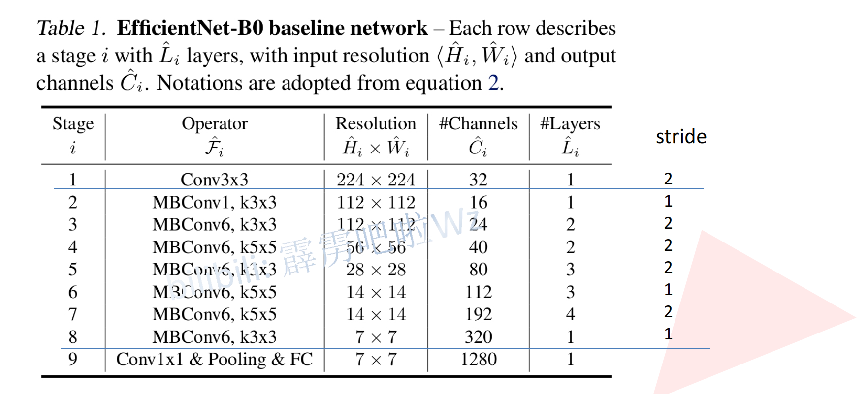
The MBConv structure is:

[1x1 dimension increase] - [DW - > se - > 1x1 [dimension decrease] - [droopout - > shortcut

SE modules are:

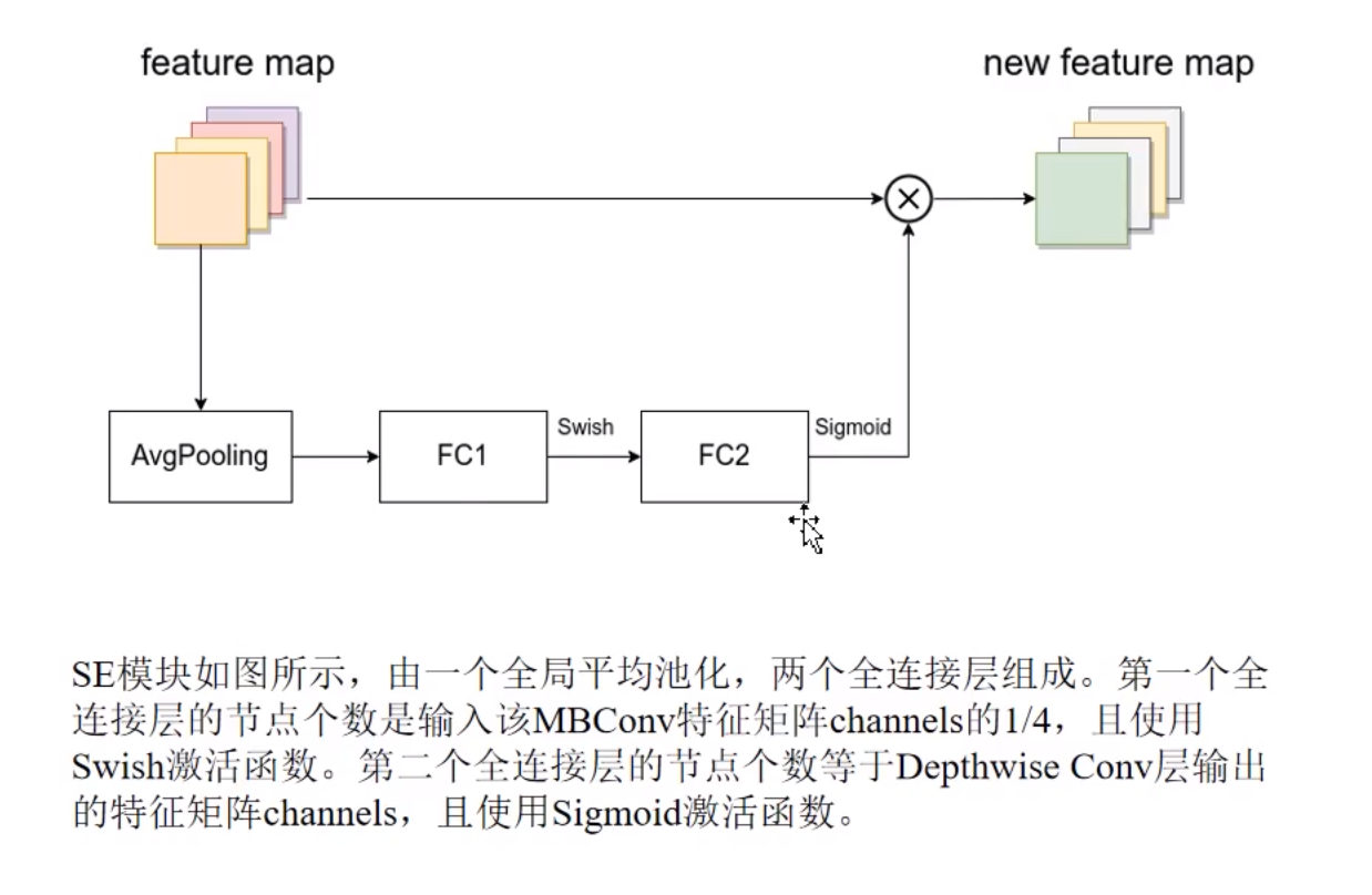
Some details:

• After the first 1x1 convolution dimension increase, the output characteristic matrix channel is n times that of the input characteristic matrix channel, and this n corresponds to the number followed by MBConv in Tabel1. When n is 1, this 1x1 convolution is actually not used (dimension increase is not required).
• The first 1x1 convolution and DW are followed by BN + Swish, while the last 1x1 dimensionality reduction convolution does not use the activation function, but the Identity function.
• The Dropout here uses the Drop path instead of the traditional Dropout.
• For the shortcut connection, it is only used if and only if the shape of the characteristic matrix of the input MBConv structure and the output characteristic matrix are the same and the strip of DW convolution = 1.

For other versions of EfficientNet, please see this table for details:

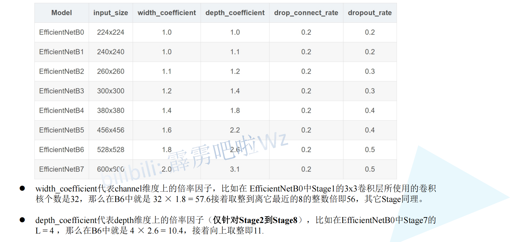
4, PyTorch recurrence

import torch.nn as nn
from typing import Optional, Callable
from torch import Tensor
from torch.nn import functional as F
from collections import OrderedDict
from functools import partial
import math
import copy
import torch


def _make_divisible(ch, divisor=8, min_ch=None):
    """
    take ch Adjust to the nearest multiple of 8
    This function is taken from the original tf repo.
    It ensures that all layers have a channel number that is divisible by 8
    It can be seen here:
    https://github.com/tensorflow/models/blob/master/research/slim/nets/mobilenet/mobilenet.py
    """
    if min_ch is None:
        min_ch = divisor
    new_ch = max(min_ch, int(ch + divisor / 2) // divisor * divisor)
    # Make sure that round down does not go down by more than 10%.
    if new_ch < 0.9 * ch:
        new_ch += divisor
    return new_ch

class ConvBNActivation(nn.Sequential):
    def __init__(self, in_planes: int, out_planes: int, kernel_size: int = 3,
                 stride: int = 1, groups: int = 1,  # Normal convolution or DW convolution
                 norm_layer: Optional[Callable[..., nn.Module]] = None,  # BN
                 activation_layer: Optional[Callable[..., nn.Module]] = None):
        padding = (kernel_size - 1) // 2
        if norm_layer is None:
            norm_layer = nn.BatchNorm2d
        if activation_layer is None:
            activation_layer = nn.SiLU   # alias Swish (torch>=1.7)
        super(ConvBNActivation, self).__init__(
            nn.Conv2d(in_channels=in_planes,
                      out_channels=out_planes,
                      kernel_size=kernel_size,
                      stride=stride,
                      padding=padding,
                      groups=groups,
                      bias=False),
            norm_layer(out_planes),
            activation_layer())

class SqueezeExcitation(nn.Module):
    def __init__(self, input_c: int, expand_c: int, squeeze_factor: int = 4):
        """
        :params input_c: MBConv Input in feature map of channel
        :params expand_c: MBConv in DW Convolution output feature map of channel=First 1 x1 After convolution dimension lifting channel
        :squeeze_factor: First full connection layer dimensionality reduction factor
        """
        super(SqueezeExcitation, self).__init__()
        squeeze_c = input_c // squeeze_ Number of nodes of factor # first full connection layer
        self.fc1 = nn.Conv2d(expand_c, squeeze_c, 1)  # Using convolution instead of full connection layer has the same dimensionality reduction effect
        self.ac1 = nn.SiLU()  # Swish
        self.fc2 = nn.Conv2d(squeeze_c, expand_c, 1)  # Ascending dimension
        self.ac2 = nn.Sigmoid()

    def forward(self, x: Tensor) -> Tensor:
        # The global average pooled attention mechanism is applied to each channel to obtain the corresponding weight of each channel
        scale = F.adaptive_avg_pool2d(x, output_size=(1, 1))
        # Then optimize the weight through continuous learning
        scale = self.fc1(scale)
        scale = self.ac1(scale)
        scale = self.fc2(scale)
        scale = self.ac2(scale)
        return scale * x

def drop_path(x, drop_prob: float = 0., traing: bool = False):
    """
    Drop paths (Stochastic Depth) per sample (when applied in main path of residual blocks).
    "Deep Networks with Stochastic Depth", https://arxiv.org/pdf/1603.09382.pdf
    This function is taken from the rwightman.
    It can be seen here:    DropBlock, DropPath
    https://github.com/rwightman/pytorch-image-models/blob/master/timm/models/layers/drop.py#L140
    """
    if drop_prob == 0. or not traing:
        return x
    keep_prob = 1 - drop_prob
    shape = (x.shape[0],) + (1,) * (x.ndim - 1)
    random_tensor = keep_prob + torch.rand(shape, dtype=x.dtype, device=x.device)
    random_tensor.floor()
    output = x.div(keep_prob) * random_tensor
    return output

class DropPath(nn.Module):
    """
    Drop paths (Stochastic Depth) per sample  (when applied in main path of residual blocks).
    "Deep Networks with Stochastic Depth", https://arxiv.org/pdf/1603.09382.pdf
    """
    def __init__(self, drop_prob=None):
        super(DropPath, self).__init__()
        self.drop_prob = drop_prob

    def forward(self, x):
        return drop_path(x, self.drop_prob, self.training)

class MBConvConfig:
    def __init__(self, kernel: int, in_planes: int, out_planes: int, expanded_ratio: int,
                 stride: int, use_se: bool, drop_rate: float, index: str, width_coefficient: float):
        """
        params: kernel: MBConv Medium DW Convoluted kernel_size(Corresponding to the in the picture k)
        params: in_planes: MBConv Module input feature map of channel
        params: out_planes: MBConv Module output feature map of channel
        params: expanded_ratio: MBConv First 1 of the module x1 Convolution layer expand_rate  Ascending dimension
        params: stride: DW Convoluted stride
        params: use_se: Whether to use se All modules are True
        params: drop_rate: MBConv Modular Dropout Random deactivation ratio of layers
        params: index: Record current MBConv Module name 1 a 2a 2b
        params: width_coefficient: Magnification factor in the direction of network width w
        """
        self.in_planes = self.adjust_channels(in_planes, width_coefficient)
        self.kernel = kernel
        self.expanded_planes = self.in_planes * expanded_ratio  # Output channel of the first 1x1 convolution layer of the MBConv module
        self.out_planes = self.adjust_channels(out_planes, width_coefficient)
        self.use_se = use_se
        self.stride = stride
        self.drop_rate = drop_rate
        self.index = index

    @staticmethod
    def adjust_channels(channels: int, width_coefficient: float):
        # Adjust the channel * width magnification factor to an integer multiple of 8
        return _make_divisible(channels * width_coefficient, 8)

class MBConv(nn.Module):
    def __init__(self, cnf: MBConvConfig, norm_layer: Callable[..., nn.Module]):
        """
        params: cnf: MBConv Layer profile
        params: norm_layer: BN structure
        """
        super(MBConv, self).__init__()
        if cnf.stride not in [1, 2]:
            raise ValueError("illegal stride value.")

        # Only the strip of DW convolution = 1 and the input channel = output channel can be shortcut connected
        self.use_shortcut = (cnf.stride == 1 and cnf.in_planes == cnf.out_planes)

        layers = OrderedDict()  # Store the structures in MBConv in turn
        activation_layer = nn.SiLU

        # Dimension upgrading of the first 1x1 convolution
        # Only when expanded_ Expanded when ratio = 1_ planes=in_ Planes, there is no dimension upgrade, so this 1x1 convolution layer is not required
        if cnf.expanded_planes != cnf.in_planes:
            layers.update({"expand_conv": ConvBNActivation(cnf.in_planes,
                                                           cnf.expanded_planes,
                                                           kernel_size=1,
                                                           norm_layer=norm_layer,  # BN
                                                           activation_layer=activation_layer)})  # Swish
        # DW convolution groups=channel
        layers.update({"dwconv": ConvBNActivation(cnf.expanded_planes,
                                                  cnf.expanded_planes,
                                                  kernel_size=cnf.kernel,
                                                  stride=cnf.stride,
                                                  groups=cnf.expanded_planes,
                                                  norm_layer=norm_layer,  # BN
                                                  activation_layer=activation_layer)})  # Swish
        # SE module
        if cnf.use_se:
            layers.update({"se": SqueezeExcitation(cnf.in_planes,
                                                   cnf.expanded_planes)})
        # Last 1x1 convolution
        layers.update({"project_conv": ConvBNActivation(cnf.expanded_planes,
                                                    cnf.out_planes,
                                                    kernel_size=1,
                                                    norm_layer=norm_layer,  # BN
                                                    activation_layer=nn.Identity)})  # Identity
        self.block = nn.Sequential(layers)
        self.out_channels = cnf.out_planes
        self.is_strided = cnf.stride > 1  # It doesn't seem to work

        # The dropout layer is used only when using a shortcut connection
        if cnf.drop_rate > 0 and self.use_shortcut:
            # self.dropout = nn.Dropout2d(p=cnf.drop_rate, inplace=True)
            self.dropout = DropPath(cnf.drop_rate)
        else:
            self.dropout = nn.Identity()

    def forward(self, x: Tensor) -> Tensor:
        result = self.block(x)
        result = self.dropout(result)
        if self.use_shortcut:
            result += x
        return result

class EfficientNet(nn.Module):
    def __init__(self, width_coefficient: float, depth_coefficient: float, num_classes: int = 1000,
                 dropout_rate: float = 0.2, drop_connect_rate: float = 0.2,
                 block: Optional[Callable[..., nn.Module]] = None,
                 norm_layer: Optional[Callable[..., nn.Module]] = None):
        """
        params: width_coefficient: The magnification factor on the network width corresponds to that in the paper w
        params: depth_coefficient: The magnification factor on the network depth corresponds to that in the paper d
        params: num_classes: Number of categories classified
        params: dropout_rate: stage9 of FC In front of the floor Dropout Random deactivation ratio
        params: drop_connect_rate: MBConv Modular Dropout The random deactivation ratio of the layer slowly increases from 0 to 0.2
        params: block: MBConv modular
        params: norm_layer: ordinary BN structure
        """
        super(EfficientNet, self).__init__()

        # B1-B7 behind the default B0 network configuration file is multiplied by the corresponding depth, width and resolution magnification factors
        # stage2 - stage8
        # kernel_size, in_channel, out_channel, exp_ratio, strides, use_SE, drop_connect_rate, repeats
        # kernel_ Size: written after mbconv knxn
        # in_channel/out_channel: the channel of the input / output feature map of the first MBConv of the current stage
        # exp_ratio: the expansion rate of the first 1x1 convolution corresponds to the current MBConvn
        # Stripes: the first of the current stage
        # use_SE: by default, each stage uses the SE module
        # drop_ connect_ Rate: the random deactivation ratio of the Dropout layer of the mbconv module is 0.2 by default and will be adjusted later
        # Repeats: the number of times mbconv is repeated in the current stage
        default_cnf = [[3, 32, 16, 1, 1, True, drop_connect_rate, 1],
                       [3, 16, 24, 6, 2, True, drop_connect_rate, 2],
                       [5, 24, 40, 6, 2, True, drop_connect_rate, 2],
                       [3, 40, 80, 6, 2, True, drop_connect_rate, 3],
                       [5, 80, 112, 6, 1, True, drop_connect_rate, 3],
                       [5, 112, 192, 6, 2, True, drop_connect_rate, 4],
                       [3, 192, 320, 6, 1, True, drop_connect_rate, 1]]

        def round_repeats(repeats):
            # depth_coefficient represents the magnification factor on the depth dimension (Stage2 to Stage8 only)
            # Use depth through this function_ The coefficient magnification factor dynamically adjusts the depth of the network (the number of repetitions of MBConv)
            return int(math.ceil(depth_coefficient * repeats))

        if block is None:
            block = MBConv

        if norm_layer is None:
            # The patial method builds a layer structure. The next time you use it, you don't need to pass the eps and momentum parameters. These two values will be passed in by default
            norm_layer = partial(nn.BatchNorm2d, eps=1e-3, momentum=0.1)

        # Use width through this function_ The coefficent magnification factor dynamically adjusts the width of the network (channel)
        # Specific method: adjust the channel * width magnification factor to an integer multiple of 8
        adjust_channels = partial(MBConvConfig.adjust_channels, width_coefficient=width_coefficient)

        # Initialize a single MB_config
        MB_config = partial(MBConvConfig, width_coefficient=width_coefficient)

        # Get the configuration information of all MB modules of stage2-stage8
        b = 0  # Used to adjust drop_connect_rate
        num_blocks = float(sum(round_repeats(i[-1]) for i in default_cnf))  # Count the number of repetitions of all MB modules
        MBConv_configs = []  # Store the configuration files of all MB modules
        for stage, args in enumerate(default_cnf):  # Traverse each stage
            cnf = copy.copy(args)
            for i in range(round_repeats(cnf.pop(-1))):  # Traverse the MB modules in each stage
                if i > 0:
                    cnf[-3] = 1  # When I > 0, stripe = 1
                    cnf[1] = cnf[2]  # When I > 0, input channel = output channel = output channel of the first MB module

                # cnf[-1] *= b / num_blocks  # update drop_connect_rate
                cnf[-1] = args[-2] * b / num_blocks
                index = str(stage + 1) + chr(i + 97)  # Record the MB structure of the current stage
                MBConv_configs.append(MB_config(*cnf, index))
                b += 1

        # Start to build the overall network structure
        layers = OrderedDict()

        # stage1
        layers.update({"stem_conv": ConvBNActivation(in_planes=3,
                                                  out_planes=adjust_channels(32),  # Adjust by width magnification factor
                                                  kernel_size=3,
                                                  stride=2,
                                                  norm_layer=norm_layer)})

        # stage2-stage8
        for cnf in MBConv_configs:
            layers.update({cnf.index: block(cnf, norm_layer)})

        # stage9
        last_conv_input_c = MBConv_configs[-1].out_planes
        last_conv_output_c = adjust_channels(1280)  # Adjust by width magnification factor
        layers.update({"top": ConvBNActivation(in_planes=last_conv_input_c,
                                                  out_planes=last_conv_output_c,
                                                  kernel_size=1,
                                                  norm_layer=norm_layer)})

        self.features = nn.Sequential(layers)
        self.avgpool = nn.AdaptiveAvgPool2d(1)

        classifier = []
        if dropout_rate > 0:
            classifier.append(nn.Dropout(p=dropout_rate, inplace=True))
        classifier.append(nn.Linear(last_conv_output_c, num_classes))
        self.classifier = nn.Sequential(*classifier)

        # Initialize weight
        for m in self.modules():
            if isinstance(m, nn.Conv2d):
                nn.init.kaiming_normal_(m.weight, mode="fan_out")
                if m.bias is not None:
                    nn.init.zeros_(m.bias)
            elif isinstance(m, nn.BatchNorm2d):
                nn.init.ones_(m.weight)
                nn.init.zeros_(m.bias)
            elif isinstance(m, nn.Linear):
                nn.init.normal_(m.weight, 0, 0.01)
                nn.init.zeros_(m.bias)

    def forward(self, x: Tensor) -> Tensor:
        x = self.features(x)
        x = self.avgpool(x)
        x = torch.flatten(x, 1)
        x = self.classifier(x)
        return x


def efficientnet_b0(num_classes=1000):
    # input image size 224x224
    return EfficientNet(width_coefficient=1.0,
                        depth_coefficient=1.0,
                        dropout_rate=0.2,
                        num_classes=num_classes)


def efficientnet_b1(num_classes=1000):
    # input image size 240x240
    return EfficientNet(width_coefficient=1.0,
                        depth_coefficient=1.1,
                        dropout_rate=0.2,
                        num_classes=num_classes)


def efficientnet_b2(num_classes=1000):
    # input image size 260x260
    return EfficientNet(width_coefficient=1.1,
                        depth_coefficient=1.2,
                        dropout_rate=0.3,
                        num_classes=num_classes)


def efficientnet_b3(num_classes=1000):
    # input image size 300x300
    return EfficientNet(width_coefficient=1.2,
                        depth_coefficient=1.4,
                        dropout_rate=0.3,
                        num_classes=num_classes)


def efficientnet_b4(num_classes=1000):
    # input image size 380x380
    return EfficientNet(width_coefficient=1.4,
                        depth_coefficient=1.8,
                        dropout_rate=0.4,
                        num_classes=num_classes)


def efficientnet_b5(num_classes=1000):
    # input image size 456x456
    return EfficientNet(width_coefficient=1.6,
                        depth_coefficient=2.2,
                        dropout_rate=0.4,
                        num_classes=num_classes)


def efficientnet_b6(num_classes=1000):
    # input image size 528x528
    return EfficientNet(width_coefficient=1.8,
                        depth_coefficient=2.6,
                        dropout_rate=0.5,
                        num_classes=num_classes)


def efficientnet_b7(num_classes=1000):
    # input image size 600x600
    return EfficientNet(width_coefficient=2.0,
                        depth_coefficient=3.1,
                        dropout_rate=0.5,
                        num_classes=num_classes)

5, Experimental results

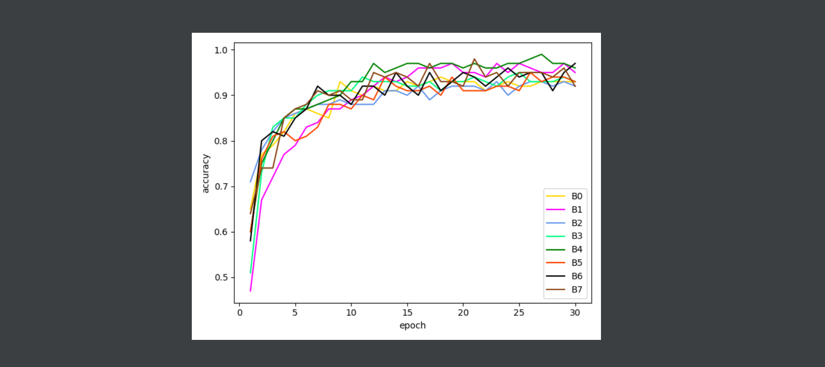
It may be a data set problem. The gap between the eight models is not large, but it can be seen that b4 is the best.