 Rimeng Society
AI AI:Keras PyTorch MXNet TensorFlow PaddlePaddle deep learning real combat (irregular update)
Parallel practice of ResNet model on GPU
Parallel practice of ResNet model on GPU
Learning objectives
- Understand the difference between model parallelism and data parallelism
- Understand the relationship between distributed training and parallel training
- Master the solution of model parallel training on single machine and multi GPU
Relevant knowledge
- Parallel / distributed training and its relationship:
- In the field of machine learning (deep learning), parallel / distributed mode is generally mainly used in the training stage of the model to accelerate the training efficiency of the model. Therefore, the method of using multi threads or multi processes of computer system to improve the efficiency of model training can be called parallel training. Among them, the way of using multi process training can also be called parallel distributed training, which is called distributed training for short (because the communication between multiple processes of a single computer is equivalent to the communication between multiple computers). Thus, distributed training is a special form of parallel training.
- Data parallel training:
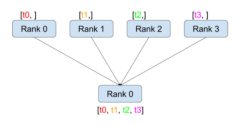
- Data parallelism is the first mock exam. Every data in training data is divided into N equal parts and sent to the same model. The model is copied to n to accept different data. After that, each model will calculate the gradient of the corresponding data, and then all the gradients are used to update the parameters of each model. Then the next batch data is parallelized (because our commonly used batch SGD optimization method is to solve the average gradient of the batch data to update the parameters).
- Model parallel training:
- Model parallelism means that the model network structure is divided into n parts, and each part will process the next batch immediately after processing a batch of data (if the model is not divided into independent parts, each part of the model must wait for all the batch of data before starting the next batch of data processing).
- This case focuses on the model parallel scheme of single machine and multi GPU to solve the problem that large models cannot be loaded on a single GPU as a whole.
Parallel model of single machine and multi GPU
- Step 1: review the hardware configuration and understand the model allocation with a simple example
- Step 2: allocate the large model ResNet50 structure to multiple GPU s
- Step 3: compare the time-consuming of multi GPU parallel and single GPU in the model
- Step 4: use pipeline technology to accelerate multi GPU training
- Step 5: find pipeline parameters to further accelerate multi GPU training
Step 1: review the hardware configuration and understand the model allocation with a simple example
- View hardware configuration
import subprocess

# Print nvidia graphics card information, including cuda version, number of graphics cards, current usage, etc
print(subprocess.check_output("nvidia-smi", universal_newlines=True))- Output effect:
# Here we can see:
# Version information of GPU Driver and CUDA
# GPU operation of two GTX1080Ti

+-----------------------------------------------------------------------------+
| NVIDIA-SMI 430.50       Driver Version: 430.50       CUDA Version: 10.1     |
|-------------------------------+----------------------+----------------------+
| GPU  Name        Persistence-M| Bus-Id        Disp.A | Volatile Uncorr. ECC |
| Fan  Temp  Perf  Pwr:Usage/Cap|         Memory-Usage | GPU-Util  Compute M. |
|===============================+======================+======================|
|   0  GeForce GTX 1080Ti  Off  | 00000000:03:00.0 Off |                  N/A |
| 20%   38C    P0    54W / 250W |      0MiB / 11178MiB |      0%      Default |
+-------------------------------+----------------------+----------------------+
|   1  GeForce GTX 1080Ti  Off  | 00000000:04:00.0 Off |                  N/A |
| 26%   45C    P0    53W / 250W |      0MiB / 11178MiB |      3%      Default |
+-------------------------------+----------------------+----------------------+

+-----------------------------------------------------------------------------+
| Processes:                                                       GPU Memory |
|  GPU       PID   Type   Process name                             Usage      |
|=============================================================================|
|  No running processes found                                                 |
+-----------------------------------------------------------------------------+
- Define a toy model with only two linear layers:
# Import the necessary toolkit for building models
import torch
import torch.nn as nn
import torch.optim as optim


class ToyModel(nn.Module):
    """Define a toy model class"""
    def __init__(self):
        super(ToyModel, self).__init__()
        # Instantiate the first linear layer (parameter) and place it on GPU '0'
        self.net1 = torch.nn.Linear(10, 10).to('cuda:0')
        # Instantiate the ReLU layer, and the parameterless calculation layer does not need any allocation
        # It doesn't occupy any storage space, it's just a calculation instruction
        self.relu = torch.nn.ReLU()
        # Instantiate the second linear layer (parameter) and place it on GPU '1'
        self.net2 = torch.nn.Linear(10, 5).to('cuda:1')

    def forward(self, x):
        # The input x needs to be multiplied by the first linear layer parameter, so it needs to be sent to GPU '0'
        # Then it is activated by the ReLU function on GPU '0'
        x = self.relu(self.net1(x.to('cuda:0')))
        # In order to continue multiplying with the second linear layer parameter, it needs to be sent to GPU '1'
        # Finally, the calculation result is returned on GPU '1'
return self.net2(x.to('cuda:1'))- Define the training configuration of the toy model:
# Instantiation model
model = ToyModel()
# Select loss function
loss_fn = nn.MSELoss()
# Select optimization method
optimizer = optim.SGD(model.parameters(), lr=0.001)

# The gradient is initialized to 0
optimizer.zero_grad()
# The output is obtained using the random tensor input model
outputs = model(torch.randn(20, 10))

# Because the result of the model is returned on GPU '1'
# Therefore, the real label should also be assigned to GPU No. 1
labels = torch.randn(20, 5).to('cuda:1')

# Calculate loss
loss_fn(outputs, labels).backward()
# Update weight
optimizer.step()
Step 2: allocate the large model ResNet50 structure to multiple GPU s
# Import the main structure of ResNet and the component unit Bottleneck of ResNet50
from torchvision.models.resnet import ResNet, Bottleneck

# The native ResNet50 output category is 1000
num_classes = 1000


class ModelParallelResNet50(ResNet):
    """In two GPU Parallel allocation on ResNet50 Model"""
    def __init__(self, *args, **kwargs):
        # Initialize a specific parameter from the ResNet main structure to become ResNet50
        # The first initialization parameter Bottleneck is a specific block unit of ResNet50
        # The second initialization parameter [3, 4, 6, 3] refers to the number of layers corresponding to the four block units of ResNet50
        # [3, 4, 6, 3] is fixed for ResNet50. If ResNet101, it corresponds to [3, 4, 23, 3]
        super(ModelParallelResNet50, self).__init__(
            Bottleneck, [3, 4, 6, 3], num_classes=num_classes, *args, **kwargs)

        # Rewrite the ResNet50 structure so that it is allocated on two GPU s
        # The internal computing layer and order are fixed
        # The first two block units (layer1, layer2) are on GPU '0'
        self.seq1 = nn.Sequential(
            self.conv1,
            self.bn1,
            self.relu,
            self.maxpool,
            self.layer1,
            self.layer2
        ).to('cuda:0')

        # The last two block units (layer3 and layer4) are on GPU '1'
        self.seq2 = nn.Sequential(
            self.layer3,
            self.layer4,
            self.avgpool,
        ).to('cuda:1')

        self.fc.to('cuda:1')

    def forward(self, x):
        # After seq1 processing, send the result to GPU '1'
        x = self.seq2(self.seq1(x).to('cuda:1'))
return self.fc(x.view(x.size(0), -1))- Define ResNet50 model training configuration:
# Define relevant configurations for model training
num_batches = 3
batch_size = 120
image_w = 128
image_h = 128


def train(model):
    """Model training function"""
    model.train(True)
    # Define loss function
    loss_fn = nn.MSELoss()
    # Define optimization method
    optimizer = optim.SGD(model.parameters(), lr=0.001)
    # Generate a tensor of [batch, 1] shape, in which each value is a random number in the [0, 1000) value range
    # This tensor will be used to generate real labels later
    one_hot_indices = torch.LongTensor(batch_size) \
                           .random_(0, num_classes) \
                           .view(batch_size, 1)

    # Start batch cycle
    for _ in range(num_batches):
        # Randomly initializes the input of the specified size
        inputs = torch.randn(batch_size, 3, image_w, image_h)
        # Initializes a zero tensor of [batch_size, num_classes]
        # Using scatter_ Method fills the tensor with values
        # The first parameter is 1, which means that it is filled in the direction of the longitudinal axis each time
        # The second parameter is one_ hot_ Indexes, which represents the position index filled in each column
        # The third parameter is 1 and the filled value is 1
        labels = torch.zeros(batch_size, num_classes) \
                      .scatter_(1, one_hot_indices, 1)

        # Gradient zeroing
        optimizer.zero_grad()
        # First, send the input to GPU '0'
        # Then call the model to get the output
        outputs = model(inputs.to('cuda:0'))

        # In order to calculate the loss, the real label needs to be sent to the device that outputs the result
        labels = labels.to(outputs.device)
        # Calculate loss on specified equipment
        loss_fn(outputs, labels).backward()
        # Update parameters according to gradient
        optimizer.step()
Step 3: compare the time-consuming of multi GPU parallel and single GPU in the model
- Draw the time-consuming diagram of model dual GPU parallel and single GPU
# Import matplotlib for drawing
import matplotlib.pyplot as plt
# Set drawing style
plt.switch_backend('Agg')

import numpy as np

# Import timeit, a time-consuming toolkit dedicated to statistical models for parallel computing
import timeit

# Set the repetition parameter of timeit. In order to highlight the difference of training time, it will be repeated 10 times
num_repeat = 10

# Set the objective function of timeit (the time consumption of this function will be calculated)
stmt = "train(model)"

# Set the startup statement of timeit, that is, the statement that runs before the calculation of time consumption starts
# The startup statement instantiates the parallel ResNet50 model
setup = "model = ModelParallelResNet50()"

# The time-consuming of ResNet50 model with 10 consecutive parallel computations
# stmt is the string form of the executed objective function
# setup is the startup statement before execution
# Number is the number of times the objective function is executed. number=1 means that the objective function is executed only once and the calculation time is spent
# Repeat is the number of times the calculation takes time. number=1, repeat=10 means that the objective function is executed once and the time is calculated;
# Repeat 10 times and get 10 results
# globals=globals() means that the code can be executed in the current global namespace, using all variables
mp_run_times = timeit.repeat(
    stmt, setup, number=1, repeat=num_repeat, globals=globals())

# Calculate the mean and standard deviation of 10 results
mp_mean, mp_std = np.mean(mp_run_times), np.std(mp_run_times)

# The startup statement is to instantiate the ResNet50 model of a single GPU
setup = "import torchvision.models as models;" + \
        "model = models.resnet50(num_classes=num_classes).to('cuda:0')"

# Calculating ResNet50 model of single GPU takes time
rn_run_times = timeit.repeat(
    stmt, setup, number=1, repeat=num_repeat, globals=globals())
# Calculate the mean and standard deviation of 10 results
rn_mean, rn_std = np.mean(rn_run_times), np.std(rn_run_times)


def plot(means, stds, labels, fig_name):
    """Drawing function"""
    # Create subgraph canvas
    fig, ax = plt.subplots()
    # Draw a histogram on the canvas and set relevant configurations
    ax.bar(np.arange(len(means)), means, yerr=stds,
           align='center', alpha=0.5, ecolor='red', capsize=10, width=0.6)
    # Set vertical axis description
    ax.set_ylabel('ResNet50 Execution Time (Second)')
    # Set horizontal axis scale
    ax.set_xticks(np.arange(len(means)))
    # Set horizontal axis scale label
    ax.set_xticklabels(labels)
    # Set y-axis gridlines
    ax.yaxis.grid(True)
    # Set layout
    plt.tight_layout()
    # Save picture
    plt.savefig(fig_name)
    # close picture
    plt.close(fig)


# Pass the corresponding parameter into the function
plot([mp_mean, rn_mean],
     [mp_std, rn_std],
     ['Model Parallel', 'Single GPU'],
'mp_vs_rn.png')- Output effect
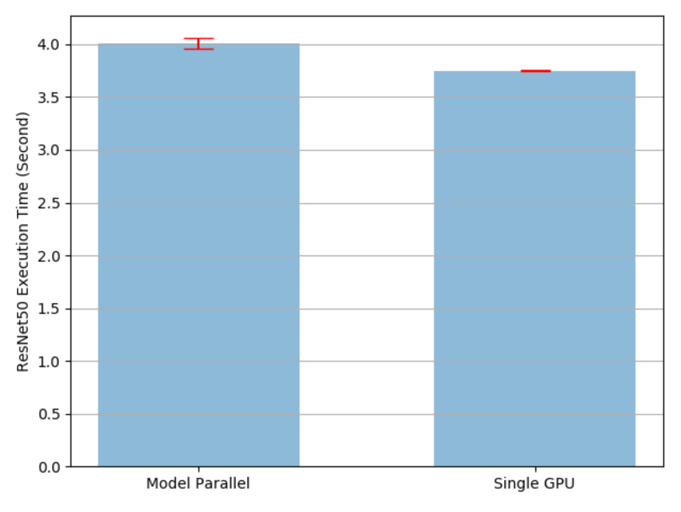
- analysis:
- It can be seen from the figure that the running time of a single GPU is less than the running time allocated by the model on two GPUs. This is because: in the current state, only one GPU works on the models on two GPUs at the same time, and they also spend time on mutual data transmission. In order to improve this situation, we will use the pipeline technology of model training, which will be explained in detail below
Step 4: use pipeline technology to accelerate multi GPU training
- Pipeline technology of model training:
- Pipeline technology aims to make the models distributed on different GPUs process the corresponding work at the same time, so as to improve the training efficiency. The principle of pipeline technology is to divide the data into N parts (n > 1), and each data is called a data heap. After the first GPU processes the first data heap, it sends the data to the second GPU. After that, the first GPU will not wait for the second GPU to complete the processing as before, but immediately process the second data heap. At this time point, both GPUs are running the corresponding work of processing until all data heaps are processed.
- The above is a standard pipeline process. A number of threads such as GPU must be started to control these asynchronous behaviors. In practical engineering, in order to avoid too high code complexity, we often do not use asynchronous processing mechanism. This is because when we divide batch data into sufficiently small data heaps, a single GPU processes them very fast, and the waiting time of other GPUs can be ignored. That is, when the second GPU processes the first data heap, it does not need to use other threads to make the first GPU process data asynchronously, but just wait for it to complete before continuing to process the second data heap. Next, we will implement the pipeline in this way and compare the results.
- Accelerate the implementation of multi GPU training using pipeline technology:
class PipelineParallelResNet50(ModelParallelResNet50):
    """Parallel model with pipeline technology ResNet50"""
    def __init__(self, split_size=20, *args, **kwargs):
        # Inheriting the initialization function of ModelParallelResNet50
        # A new initialization parameter split is added_ Size represents the size of each batch data division
        # Such as batch_size=120, split_size=20 indicates that 120 pieces of data are divided into 6 copies,
        # Number of 20 pieces per piece processed as pipeline
        super(PipelineParallelResNet50, self).__init__(*args, **kwargs)
        self.split_size = split_size

    def forward(self, x):
        """Rewrite pipelined forward function"""
        # Divide the input batch data according to split_size partition and encapsulated with iterators
        splits = iter(x.split(self.split_size, dim=0))
        # Use the next method to fetch the first data (the first data heap) in the iterator
        s_next = next(splits)
        # The data is processed on GPU '0' and sent to GPU '1'
        s_prev = self.seq1(s_next).to('cuda:1')
        # Create a list that stores the final processing results
        ret = []

        # Loop through all data heaps in the iterator
        for s_next in splits:
            # Processing data from GPU '0' on GPU '1'
            s_prev = self.seq2(s_prev)
            # Input the result view into the specified dimension to the full connection layer
            # Finally, load the result list
            ret.append(self.fc(s_prev.view(s_prev.size(0), -1)))
            # Continue to process the data on GPU '0' and send it to GPU '1'
            s_prev = self.seq1(s_next).to('cuda:1')

        # When the last data heap loop traversal is completed, it is only sent to GPU '1' and not processed
        # Therefore, the processing should be completed on GPU '1'
        s_prev = self.seq2(s_prev)
        # Similarly, input the result view into the specified dimension to the full connection layer
        # Finally, load the result list
        ret.append(self.fc(s_prev.view(s_prev.size(0), -1)))
        # Returns the tensor form of the result
        return torch.cat(ret)


# The startup statement instantiates the multi GPU parallel ResNet50 model with pipeline
setup = "model = PipelineParallelResNet50()"

# timeit is used for time-consuming calculation, and the parameters are the same as those used above
pp_run_times = timeit.repeat(
    stmt, setup, number=1, repeat=num_repeat, globals=globals())
# Calculate the mean and standard deviation
pp_mean, pp_std = np.mean(pp_run_times), np.std(pp_run_times)

# Draw time-consuming comparison chart
plot([mp_mean, rn_mean, pp_mean],
     [mp_std, rn_std, pp_std],
     ['Model Parallel', 'Single GPU', 'Pipelining Model Parallel'],
'mp_vs_rn_vs_pp.png')- Output effect
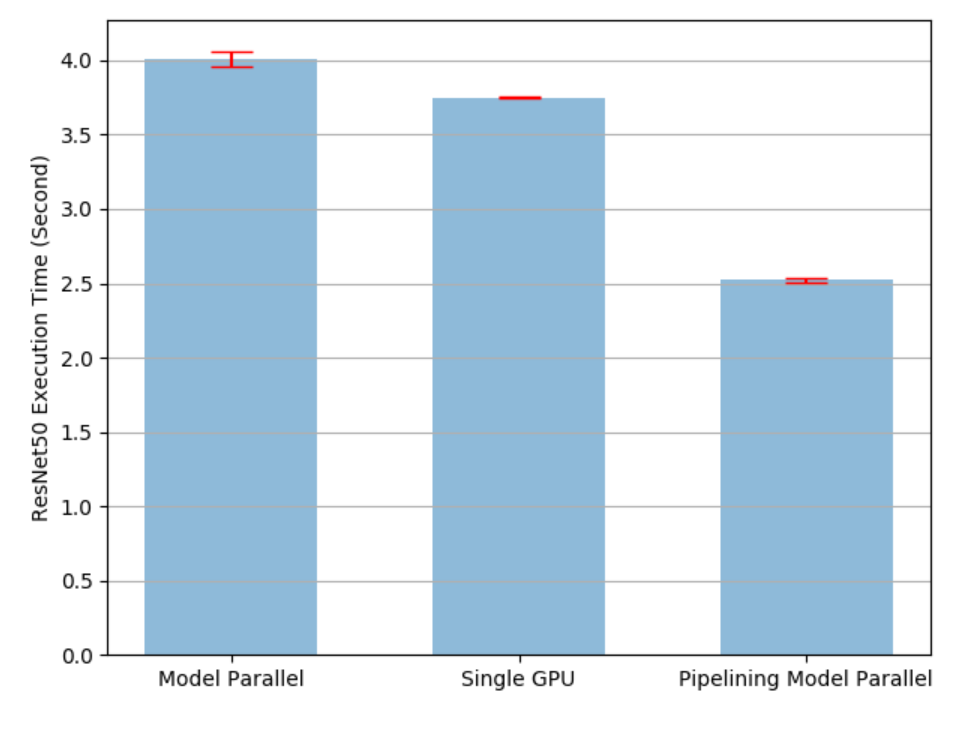
- analysis:
- It can be seen from the figure that the model training with pipeline technology takes the shortest time (running time), which has been significantly improved compared with single GPU operation. However, we find that pipelining technology introduces a new parameter split_size, which represents the size of the data heap, also directly affects the time-consuming of model training. We can use two extreme examples to explain this effect when split_size and batch_ When the size is the same, that is, the equivalent is the case without pipeline, which takes more time than a single GPU. And when split_ When size = 1, although the calculation time and waiting time are small enough, the data transmission time between GPUs will be enlarged, resulting in longer training time. Next, we will find the best split from the experiment_ size
- Step 5: find pipeline parameters to further accelerate multi GPU training
# Create a list that stores the mean and standard deviation
means = []
stds = []

# Set a set of split_ Sample point for size
split_sizes = [1, 3, 5, 8, 10, 12, 20, 40, 60]

# Traverse sampling points
for split_size in split_sizes:
    # The startup statement instantiates the multi GPU parallel ResNet50 model with pipeline
    setup = "model = PipelineParallelResNet50(split_size=%d)" % split_size
    # Use timeit to calculate the time consumption of each sampling point
    pp_run_times = timeit.repeat(
        stmt, setup, number=1, repeat=num_repeat, globals=globals())
    # Save mean and standard deviation
    means.append(np.mean(pp_run_times))
    stds.append(np.std(pp_run_times))

# Create canvas
fig, ax = plt.subplots()
# Draw mean curve
ax.plot(split_sizes, means)
# Plot the fluctuation range (standard deviation) of the mean point
ax.errorbar(split_sizes, means, yerr=stds, ecolor='red', fmt='ro')
# Set the abscissa and ordinate name
ax.set_ylabel('ResNet50 Execution Time (Second)')
ax.set_xlabel('Pipeline Split Size')
# Set scale
ax.set_xticks(split_sizes)
# Set grid display
ax.yaxis.grid(True)
# Set layout
plt.tight_layout()
# Save picture
plt.savefig("split_size_tradeoff.png")
# Close canvas
plt.close(fig)- Output effect
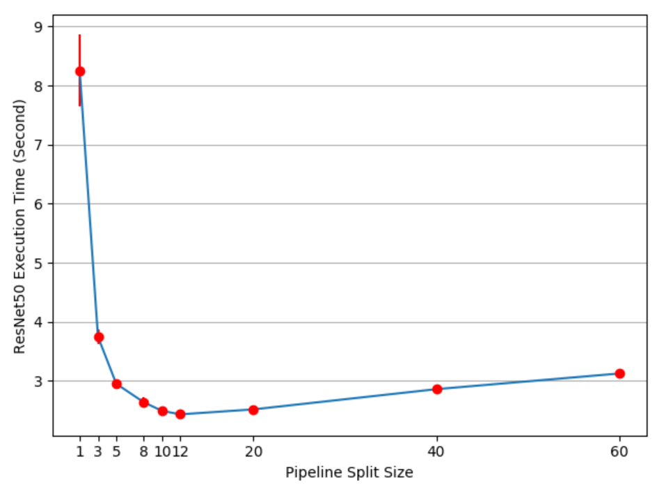
- analysis:
- As can be seen from the figure, the best split_size is 12, which takes the shortest time. If you continue to reduce split_size, the data transmission time between hardware will increase significantly. Therefore, when using model parallel pipeline technology, we should first find the appropriate split through the sampling point_ The size value is used as the parameter, and then the model parallel training is carried out