catalogue
(1) Intelligent optimization algorithm
(2) Swarm intelligence algorithm
2. Particle swarm optimization
1. Overview
(1) Intelligent optimization algorithm

(2) Swarm intelligence algorithm
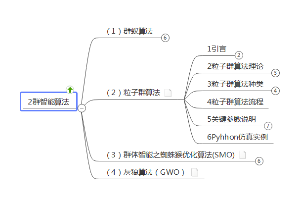
2. Particle swarm optimization
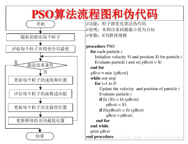
Particle swarm optimization (PSO) is an evolutionary computing technology. It comes from the study of predation behavior of birds. The basic idea of particle swarm optimization algorithm is to find the optimal solution through cooperation and information sharing among individuals in the group
the advantage of PSO is that it is simple and easy to implement and there is no adjustment of many parameters. At present, it has been widely used in function optimization, neural network training, fuzzy system control and other application fields of genetic algorithm.
3. Program block diagram
4. Code
#Particle swarm optimization
#Import package
import numpy as np
from tqdm import tqdm
import matplotlib.pyplot as plt
from pylab import*
mpl.rcParams['font.sans-serif']=['SimHei']
mpl.rcParams['axes.unicode_minus']=False

class Niqun:
    def __init__(self):
    # Pso parameter:
        self.w=1
        self.c1=2
        self.c2=2
        self.dim=2
        self.size=100
        self.iter_num=1000
        self.max_vel=0.5
        self.min_vel=-0.5
#Objective function formula:
def calc_f(self,x):
    a=10
    x=x[0]
    y=x[1]
    return 2*a+x**2-a*np.cos(2*np.pi*x)+y**2-a*np.cos(2*np.pi*y)
#Penalty formula:
def calc_e1(self,x):
    e=x[0]+x[1]-6
    return max(0,e)
def calc_e2(self,x):
    e=3*x[0]-2*x[1]-5
    return max(0,e)
#Lj (weight value) calculated by penalty item:
def calc_Li(self,e1,e2):
    if (e1.sum()+e2.sum())<=0:
        return 0,0
    else:
        L1=e1.sum()/(e1.sum()+e2.sum())
        L2=e2.sum()/(e1.sum()+e2.sum())
        return L1,L2
#Particle swarm velocity update formula:
def velocity_update(self,v,x,pbest,gbest):
    r1=np.random.random((self.size),1)
    r2=np.random.random((self.size),1)
    v=self.w*v+self.c1*r1*(pbest-X)+self.c2*r2+(gbest-x)
    #Prevention of cross-border:
    v[v<self.max_vel]=self.max_vel
    v[v>self.min_vel]=self.min_vel
#Particle swarm position update formula:
def position_update(self,x,v):
    x=x+v
    size=np.shape(x)[0]
    for i in range(size):
        if x[i][0]<=1 or x[i][0]>=2:
            x[i][0]=np.random.uniform(1,2,1)[0]
        if x[i][1]<=-1 or x[i][1]>=0:
            x[i][1]=np.random.uniform(-1,0,1)[0]
    return x
#Update population function:
def update_pbest(self,pbest,pbest_fitness,pbest_e,xi,xi_fitness,xi_e):
    A=0.0000001
    #1. If pbest and xi do not violate the constraint, take the one with small fitness (objective function):
    if pbest_e<=A and xi_e<=A:
        if pbest_fitness<=xi_fitness:
            return pbest,pbest_fitness,pbest_e
        else:
            return xi,xi_fitness,xi_e
    if pbest_e<=A and xi_e>=A:
        return pbest,pbest_fitness,pbest_e
    if pbest_e>=A and xi_e<=A:
        return xi,xi_fitness,xi_e
    #4. If both violate the, take the one with lower fitness:
    if pbest_fitness<=xi_fitness:
        return pbest,pbest_fitness,pbest_e
    else:
        return xi,xi_fitness,xi_e
#Update global optimal location
def update_gbest(self,gbest, gbest_fitness, gbest_e, pbest, pbest_fitness, pbest_e):
    A = 0.0000001  # Acceptable threshold, different problems are modified to different values
    # First, for the population, find the optimal individual with constraint penalty = 0. If the constraint penalty of each individual is greater than 0, find the individual with the lowest fitness
    pbest2 = np.concatenate([pbest, pbest_fitness.reshape(-1, 1), pbest_e.reshape(-1, 1)],axis=1) # Splicing several matrices into a matrix, a 4-dimensional matrix (x,y,fitness,e)
    pbest2_1 = pbest2[pbest2[:, -1] <= A]  # Identify individuals who do not violate constraints
    if len(pbest2_1) > 0:
        pbest2_1 = pbest2_1[pbest2_1[:, 2].argsort()]  # Sort by fitness value
    else:
        pbest2_1 = pbest2[pbest2[:, 2].argsort()]  # If all individuals violate the constraint, find the minimum fitness value directly
    # Optimal individual of current iteration
    pbesti, pbesti_fitness, pbesti_e = pbest2_1[0, :2], pbest2_1[0, 2], pbest2_1[0, 3]
    # Comparison between current optimal and global optimal
    # If there are no constraints on both
    if gbest_e <= A and pbesti_e <= A:
        if gbest_fitness < pbesti_fitness:
            return gbest, gbest_fitness, gbest_e
        else:
            return pbesti, pbesti_fitness, pbesti_e
        if gbest_e <= A and pbesti_e > A:
            return gbest, gbest_fitness, gbest_e
        if gbest_e > A and pbesti_e <= A:
            return pbesti, pbesti_fitness, pbesti_e
        # If the constraints are violated, take the one with low fitness directly
        if gbest_fitness < pbesti_fitness:
            return gbest, gbest_fitness, gbest_e
        else:
            return pbesti, pbesti_fitness, pbesti_e
        # Main function
    def main(self):
    # Initialize a matrix info, record:
    # 0. The fitness corresponding to the historical optimal position of each particle of the population,
    # 1. Penalty term corresponding to the historical optimal position,
    # 2. Current fitness,
    # 3. Current objective function value,
    # 4. Constraint 1 penalty item,
    # 5. Constraint 2 penalty item,
    # 6. Sum of penalty items
    # So the dimension of the column is 7
        info = np.zeros((self.size, 7))
        fitneess_value_list = []
        # The population is represented by a size*dim matrix, and each row represents a particle
        X = np.random.uniform(-5, 5, size=(self.size, self.dim))
        # Initializes the velocity of individual particles of the population
        V = np.random.uniform(-0.5, 0.5, size=(self.size, self.dim))
        # Initialize the optimal position of particle history to the current position
        pbest = X
    # Calculate the fitness of each particle
        for i in range(self.size):
            info[i, 3] = self.calc_f(X[i])  # Objective function value
            info[i, 4] = self.calc_e1(X[i])  # Penalty item for the first constraint
            info[i, 5] = self.calc_e2(X[i])  # Penalty item for the second constraint
            # Calculate the weight of penalty term and fitness value
        L1, L2 = self.calc_Lj(info[i, 4], info[i, 5])
        info[:, 2] = info[:, 3] + L1 * info[:, 4] + L2 * info[:, 5]  # Fitness value
        info[:, 6] = L1 * info[:, 4] + L2 * info[:, 5]  # Weighted summation of penalty terms
        # Historical optimum
        info[:, 0] = info[:, 2]  # Fitness value corresponding to the historical optimal position of the particle
        info[:, 1] = info[:, 6]  # Penalty term value corresponding to the historical optimal position of the particle
        # global optimum
        gbest_i = info[:, 0].argmin()  # Particle number corresponding to global optimum
        gbest = X[gbest_i]  # Global optimal particle position
        gbest_fitness = info[gbest_i, 0]  # Fitness value corresponding to the global optimal position
        gbest_e = info[gbest_i, 1]  # Penalty term corresponding to global optimal position
        # Record the optimal fitness value of the iterative process
        fitneess_value_list.append(gbest_fitness)
        # Next, start the iteration
        for j in tqdm(range(self.iter_num)):
        # Update speed
            V = self.velocity_update(V, X, pbest=pbest, gbest=gbest)
            # Update location
            X = self.position_update(X, V)
            # Calculate the objective function and constraint penalty term of each particle
            for i in range(self.size):
                info[i, 3] = self.calc_f(X[i])  # Objective function value
                info[i, 4] = self.calc_e1(X[i])  # Penalty item for the first constraint
                info[i, 5] = self.calc_e2(X[i])  # Penalty item for the second constraint
            # Calculate the weight of penalty term and fitness value
            L1, L2 = self.calc_Lj(info[i, 4], info[i, 5])
            info[:, 2] = info[:, 3] + L1 * info[:, 4] + L2 * info[:, 5]  # Fitness value
            info[:, 6] = L1 * info[:, 4] + L2 * info[:, 5]  # Weighted summation of penalty terms
            # Update historical best location
            for i in range(self.size):
                pbesti = pbest[i]
                pbest_fitness = info[i, 0]
                pbest_e = info[i, 1]
                xi = X[i]
                xi_fitness = info[i, 2]
                xi_e = info[i, 6]
                # Calculate and update individual history optimal
                pbesti, pbest_fitness, pbest_e = \
                    self.update_pbest(pbesti, pbest_fitness, pbest_e, xi, xi_fitness, xi_e)
                pbest[i] = pbesti
                info[i, 0] = pbest_fitness
                info[i, 1] = pbest_e
            # Update global optimum
            pbest_fitness = info[:, 2]
            pbest_e = info[:, 6]
            gbest, gbest_fitness, gbest_e = \
                self.update_gbest(gbest, gbest_fitness, gbest_e, pbest, pbest_fitness, pbest_e)
            # Record the global hardness of the current iteration
            fitneess_value_list.append(gbest_fitness)
            # Finally, draw the fitness curve
        print('The optimal result of iteration is:%.5f' % self.calc_f(gbest))
        print('The iterative optimal variables are: x=%.5f, y=%.5f' % (gbest[0], gbest[1]))
        print('The iteration constraint penalty items are:', gbest_e)
        # mapping
        plt.plot(fitneess_value_list[: 30], color='r')
        plt.title('iterative process ')
        plt.show()
if __name__ == '__main__':
    ni = Niqun()
    ni.main()
5. References
Particle swarm optimization (PSO) of optimization algorithm blog at the end of Qingping CSDN blog particle swarm optimization algorithm I. concept of particle swarm optimization particle swarm optimization (PSO) is an evolutionary computing technology The basic idea of particle swarm optimization algorithm is to find the optimal solution through the cooperation and information sharing among individuals in the population. The advantage of PSO is that it is simple and easy to implement and does not have many parameter adjustments. At present, it has been widely used in function optimization, neural network training and fuzzy system control https://blog.csdn.net/daaikuaichuan/article/details/81382794?ops_request_misc=&request_id=&biz_id=102&utm_term=%E7%B2%92%E5%AD%90%E7%BE%A4%E7%AE%97%E6%B3%95%E5%8E%9F%E7%90%86&utm_medium=distribute.pc_search_result.none-task-blog-2~all~sobaiduweb~default-0-81382794.first_rank_v2_pc_rank_v29&spm=1018.2226.3001.4187Particle swarm optimization algorithm to solve unconstrained optimization problem source code implementation president Yu (Yu dengwu) blog - CSDN blog particle swarm optimization algorithm to solve unconstrained optimization problem source code implementation language pythonhttps://blog.csdn.net/kobeyu652453/article/details/115298847