1. Introduction to algorithm

Particle swarm optimization The idea of is derived from the study of bird predation behavior, which simulates the flight and foraging behavior of bird clusters, and makes the group achieve the optimal purpose through collective cooperation. Imagine a scenario where a group of birds are randomly searching for food. There is a piece of food in an area. All birds do not know where the food is, but they can feel how far away the current position is from the food. What is the optimal strategy to find the food at this time? The answer is: search the area around the bird nearest to the food, and judge the location of the food according to your flight experience.

PSO is inspired by this model: 1. The solution of each optimization problem is imagined as a bird, called 'particles', and all particles search in a D-dimensional space. 2. 2. The fitness value of all particles is determined by a fitness function to judge the current position. 3. Each particle is endowed with memory function and can remember the best position searched. 4. Each particle also has a speed to determine the distance and direction of flight. This speed is dynamically adjusted according to its own flight experience and the flight experience of its companions. 5. It can be seen that the basis of particle swarm optimization algorithm is the social sharing of = = information==

In D-dimensional space, there are N particles; Particle i position: xi=(xi1,xi2,... xiD), substitute Xi into the fitness function f(xi) to find the fitness value; Particle i velocity: vi=(vi1,vi2,... viD) best position experienced by particle i individual: pbesti=(pi1,pi2,... piD) best position experienced by population: gbest=(g1,g2,... gD)

Generally, the position variation range in the D (1 ≤ D ≤ d) dimension is limited to ($X {min, D}, X {max, D} $),
The speed variation range is limited to ($- V {max, D}, V {max, D} $) (i.e. in the iteration, if
If the boundary value is exceeded, the speed or position of the dimension is limited to the maximum speed or boundary of the dimension
Location)   Update formula of speed and position   With the above understanding, a key problem is how to update the velocity and position of particles?

d-dimensional velocity update formula of particle i:

d-dimensional position update formula of particle i

$v_{id}^k $: the d-dimensional component $X of the flight velocity vector of particle i in the k-th iteration_ {ID} ^ k $: the d-dimensional components c1,c2 of the particle i position vector in the k-th iteration: acceleration constant, adjust the maximum learning step (hyperparameter) r1,r2: two random functions, value range [0,1] to increase randomness, w: inertia weight, non negative number, and adjust the search range of the solution space. (hyperparameters) it can be seen that pso algorithm contains three hyperparameters.

The particle velocity update formula is introduced here:

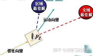
Its velocity update formula includes three parts: the first part is the previous velocity of particles   The second part is the "cognition" part, which represents the thinking of the particle itself, which can be understood as the distance between the current position of particle i and its best position. The third part is the "social part", which represents the information sharing and cooperation between particles, which can be understood as the distance between the current position of particle i and the best position of the group. As shown in the figure below, the motion process of particles is affected by the above three aspects:

2. Algorithm flow

1. Initial:  Initialize particles Population (population size n), including random location and speed.
2. Evaluation: evaluate the fitness of each particle according to the fitness function.
3. Find the Pbest: for each particle, compare its current fitness value with the fitness value corresponding to its individual historical best position (pbest). If the current fitness value is higher, the historical best position pbest will be updated with the current position.
4. Find the Gbest: for each particle, compare its current fitness value with the fitness value corresponding to the global best position (gbest). If the current fitness value is higher, the global best position gbest will be updated with the position of the current particle.
5. Update the Velocity: updates the velocity and position of each particle according to the formula.
6. If the end condition is not met, return to step 2. Usually, when the algorithm reaches the maximum number of iterations or the increment of the best fitness value is less than a given threshold, the algorithm stops.

The flow chart of the algorithm is as follows:

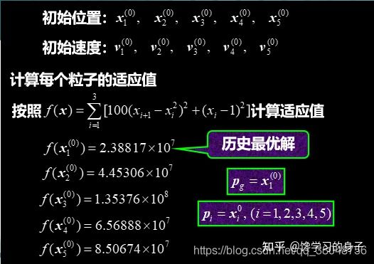
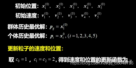
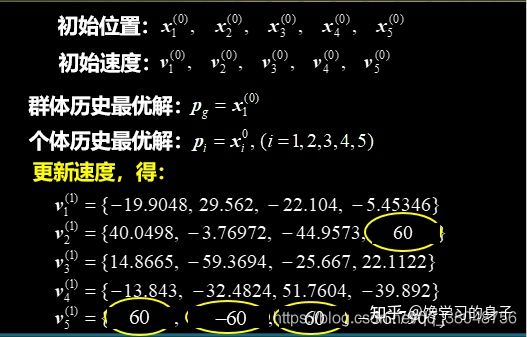
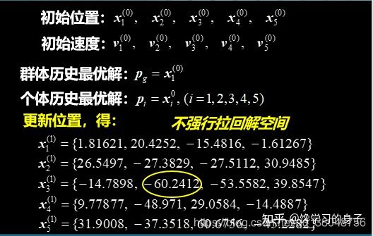
3. Algorithm example

4. Algorithm implementation

Taking the above example as an example, the implementation of the algorithm is as follows. If you need to optimize other problems, you only need to adjust the fitness function.

import numpy as np
import matplotlib.pyplot as plt
from mpl_toolkits.mplot3d import Axes3D


def fit_fun(x):  # Fitness function
    return sum(100.0 * (x[0][1:] - x[0][:-1] ** 2.0) ** 2.0 + (1 - x[0][:-1]) ** 2.0)


class Particle:
    # initialization
    def __init__(self, x_max, max_vel, dim):
        self.__pos = np.random.uniform(-x_max, x_max, (1, dim))  # Position of particles
        self.__vel = np.random.uniform(-max_vel, max_vel, (1, dim))  # Particle velocity
        self.__bestPos = np.zeros((1, dim))  # The best position for particles
        self.__fitnessValue = fit_fun(self.__pos)  # Fitness function value

    def set_pos(self, value):
        self.__pos = value

    def get_pos(self):
        return self.__pos

    def set_best_pos(self, value):
        self.__bestPos = value

    def get_best_pos(self):
        return self.__bestPos

    def set_vel(self, value):
        self.__vel = value

    def get_vel(self):
        return self.__vel

    def set_fitness_value(self, value):
        self.__fitnessValue = value

    def get_fitness_value(self):
        return self.__fitnessValue


class PSO:
    def __init__(self, dim, size, iter_num, x_max, max_vel, tol, best_fitness_value=float('Inf'), C1=2, C2=2, W=1):
        self.C1 = C1
        self.C2 = C2
        self.W = W
        self.dim = dim  # Dimension of particles
        self.size = size  # Number of particles
        self.iter_num = iter_num  # Number of iterations
        self.x_max = x_max
        self.max_vel = max_vel  # Maximum particle velocity
        self.tol = tol  # Cut off condition
        self.best_fitness_value = best_fitness_value
        self.best_position = np.zeros((1, dim))  # Optimal position of population
        self.fitness_val_list = []  # Optimal fitness per iteration

        # Initialize the population
        self.Particle_list = [Particle(self.x_max, self.max_vel, self.dim) for i in range(self.size)]

    def set_bestFitnessValue(self, value):
        self.best_fitness_value = value

    def get_bestFitnessValue(self):
        return self.best_fitness_value

    def set_bestPosition(self, value):
        self.best_position = value

    def get_bestPosition(self):
        return self.best_position

    # Update speed
    def update_vel(self, part):
        vel_value = self.W * part.get_vel() + self.C1 * np.random.rand() * (part.get_best_pos() - part.get_pos()) \
                    + self.C2 * np.random.rand() * (self.get_bestPosition() - part.get_pos())
        vel_value[vel_value > self.max_vel] = self.max_vel
        vel_value[vel_value < -self.max_vel] = -self.max_vel
        part.set_vel(vel_value)

    # Update location
    def update_pos(self, part):
        pos_value = part.get_pos() + part.get_vel()
        part.set_pos(pos_value)
        value = fit_fun(part.get_pos())
        if value < part.get_fitness_value():
            part.set_fitness_value(value)
            part.set_best_pos(pos_value)
        if value < self.get_bestFitnessValue():
            self.set_bestFitnessValue(value)
            self.set_bestPosition(pos_value)

    def update_ndim(self):

        for i in range(self.iter_num):
            for part in self.Particle_list:
                self.update_vel(part)  # Update speed
                self.update_pos(part)  # Update location
            self.fitness_val_list.append(self.get_bestFitnessValue())  # After each iteration, the current Optimal fitness Save to list
            print('The first{}The next best fitness is{}'.format(i, self.get_bestFitnessValue()))
            if self.get_bestFitnessValue() < self.tol:
                break

        return self.fitness_val_list, self.get_bestPosition()

if __name__ == '__main__':
    # test banana function
    pso = PSO(4, 5, 10000, 30, 60, 1e-4, C1=2, C2=2, W=1)
    fit_var_list, best_pos = pso.update_ndim()
    print("Optimal location:" + str(best_pos))
    print("Optimal solution:" + str(fit_var_list[-1]))
    plt.plot(range(len(fit_var_list)), fit_var_list, alpha=0.5)

5. Algorithm application

Note that the algorithm needs to pay attention to the following points when solving specific problems:   1. Population size m   m is very small, it is easy to fall into local optimization, m is very large, and the optimization ability of pso is very good. When the population number increases to a certain level, re growth will no longer play a significant role.   2. Weight factor   For the three parts of particle velocity update: A. inertia factor w=1 indicates the basic particle swarm optimization algorithm, and w=0 indicates the loss of velocity memory of the particle itself. b. The learning factor c1=0 in the self cognition part indicates that the selfless particle swarm optimization algorithm has only society and no self, which will make the group lose diversity, which is easy to fall into local optimization and can not jump out. c. The learning factor c2=0 of the social experience part indicates that the self particle swarm optimization algorithm has only self and no society, which leads to no social sharing of information and slow convergence speed of the algorithm. The selection of these three parameters is very important. How to adjust these three parameters so that the algorithm can avoid premature and converge faster is of great significance to solve practical problems.   3. Maximum speed   The function of speed limit is to maintain the balance between the exploration ability and development ability of the algorithm$ V_ When m $is large, it has strong exploration ability, but particles are easy to fly Optimal solution  $ V_m $is small and has strong development ability, but it is easy to fall into the local optimal solution $V_m $is generally set to 10% ~ 20% of the variation range of each dimensional variable   4. Cessation criteria   a. Maximum number of iterations b. acceptable satisfactory solution (judge whether it is satisfactory through fitness function)   5. Initialization of particle space   Better selection of the initialization space of particles will greatly shorten the convergence time. The initialization space is set according to specific problems. The setting of a few key parameters of the algorithm has a significant impact on the accuracy and efficiency of the algorithm   six Linear decreasing weight (not measured)

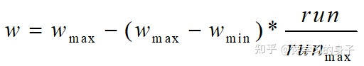
$w_{max}$Maximum inertia weight，$w_{min}$Minimum inertia weight , run, current iterations, $run_{max} $is the total number of algorithm iterations

The larger w has better global convergence ability, and the smaller w has stronger local convergence ability. Therefore, with the increase of the number of iterations, the inertia weight W should be reduced continuously, so that the particle swarm optimization algorithm has strong global convergence ability in the initial stage and strong local convergence ability in the later stage.   7. Shrinkage factor method (not measured)

In 1999, Clerc introduced the contraction factor to ensure the convergence of the algorithm, that is, the speed update formula was changed to the above formula, in which the contraction factor K was affected φ one φ 2 restricted w. φ one φ 2 is the model parameter that needs to be preset.

The contraction factor method controls the final convergence of the system behavior, and can effectively search different regions. This method can obtain high-quality solutions.   8. Neighborhood topology of the algorithm (not measured)   The neighborhood topology of particle swarm optimization algorithm includes two kinds: one is to take all individuals in the population as the neighborhood of particles, and the other is to take only some individuals in the population as the neighborhood of particles. The neighborhood topology determines the historical optimal position of the population, so the algorithm is divided into Global particle swarm optimization And local particle swarm optimization, the above I implemented is the global particle swarm optimization algorithm. Global particle swarm optimization algorithm 1. The historical optimal value of the particle itself 2. The global optimal value of the particle swarm local particle swarm optimization algorithm 1. The historical optimal value of the particle itself 2. The optimal value neighborhood of the particle in the particle neighborhood increases linearly with the increase of the number of iterations, and finally the neighborhood extends to the whole particle swarm. Practice shows that the global version of particle swarm optimization has fast convergence speed, but it is easy to fall into local optimization. The local version of particle swarm optimization algorithm has slow convergence speed, but it is difficult to fall into local optimization. Nowadays, most particle swarm optimization algorithms work hard in two aspects: convergence speed and getting rid of local optimization. In fact, these two aspects are contradictory. See how to better compromise.