1, Introduction to grey Wolf algorithm

Grey wolf optimization algorithm (Grey Wolf Optimizer, GWO) a population intelligent optimization algorithm proposed by Mirjalili, a scholar at Griffith University in Australia, in 2014. The algorithm is an optimization search method inspired by the prey hunting activities of gray wolves. It has the characteristics of strong convergence, few parameters and easy implementation. In recent years, it has attracted extensive attention of scholars and has been widely used as an optimization search method It has been successfully applied to the fields of job shop scheduling, parameter optimization, image classification and so on.

Algorithm principle:

Gray wolf belongs to the social canine family and is at the top of the food chain. Gray wolves strictly abide by a hierarchy of social dominance. As shown in the figure:

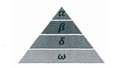
The first level of social hierarchy: the first wolf in the wolf pack is recorded as ， Wolves are mainly responsible for making decisions on predation, habitat, work and rest time and other activities. Because other wolves need to obey Wolf orders, so Wolves are also called dominant wolves. In addition, Wolves are not necessarily the strongest wolves in the pack, but in terms of management ability, The wolf must be the best.

Social class level 2: Wolf, it obeys Wolf, and assist Wolves make decisions. stay When wolves die or grow old, The wolf will be The best candidate for the wolf. although Wolf obedience Wolf, but Wolves can dominate wolves at other social levels.

Social class level 3: Wolf, it obeys , Wolves, which dominate the remaining levels at the same time. Wolves are generally composed of young wolves, sentinel wolves, hunting wolves, old wolves and nursing wolves.

Social class level 4: Wolf, it usually needs to obey wolves at other social levels. Although it seems Wolves don't play a big role in wolves, but if they don't With the existence of wolves, wolves will have internal problems, such as killing each other.

GWO optimization process includes the steps of gray wolf's social hierarchy, tracking, encircling and attacking prey. The specific steps are as follows.

1) Social Hierarchy when designing GWO, it is first necessary to build a gray wolf Social Hierarchy model. Calculate the fitness of each individual in the population, and mark the three gray wolves with the best fitness in the wolf group as , , , and the remaining gray wolves are marked . In other words, the social rank of gray wolf group is from high to low; , , and . The optimization process of GWO is mainly composed of the best three solutions in each generation of population (i.e , , )To guide the completion.

2) Encircling Prey the grey wolf will gradually approach the prey and encircle it. The mathematical model of this behavior is as follows:

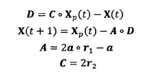
Where: t is the current number of iterations:. express hadamard product Operation; A and C are synergy coefficient vectors; Xp represents the position vector of prey; X(t) represents the position vector of the current gray wolf; In the whole iterative process, a decreases linearly from 2 to 0; r1 and r2 are random vectors in [0, 1].

3) Hunting

Gray wolf has the ability to identify the location of potential prey (optimal solution), and the search process mainly depends on , , With the guidance of the gray wolf. However, the solution space characteristics of many problems are unknown, and the gray wolf can not determine the exact location of prey (optimal solution) , , It has strong ability to identify the location of potential prey. Therefore, during each iteration, the best three gray wolves in the current population are retained( , , )And then update other search agents (including )The location of the. The mathematical model of this behavior can be expressed as follows:

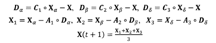
Where:,, Each represents the current population , , Position vector of; X represents the position vector of gray wolf;,, Respectively represent the distance between the current candidate gray wolf and the best three wolves; When ｜ > 1, gray wolves disperse in various areas and search for prey as much as possible. When ｜ < 1, the gray wolf will concentrate on the prey in one or some areas.

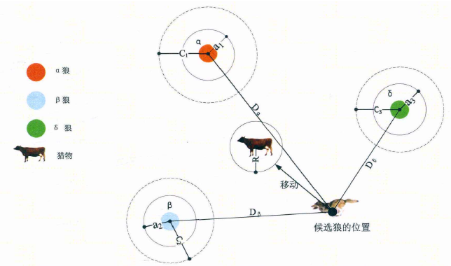
As can be seen from the figure, the position of the candidate solution finally falls on the target , , Defined random circle position. in general, , , First, the approximate location of the prey (potential optimal solution) needs to be predicted, and then other candidate wolves randomly update their location near the prey under the guidance of the current optimal Blue Wolf.

4) In the process of constructing the attack prey model, according to the formula in 2), the decrease of a value will cause the value of a to fluctuate. In other words, a is an interval [- a,a] (Note: in the first paper of the original author, this is [- 2a,2a], which is corrected as [- a,a]), where a decreases linearly in the iterative process. When a is in the interval [- 1, 1], the next position of the Search Agent can be anywhere between the current gray wolf and the prey.

5) Gray wolves mainly rely on hunting for prey , , To find prey. They began to search for prey location information scattered, and then concentrated to attack prey. For the establishment of the decentralized model, the search agent is kept away from the prey by ｜ > 1. This search method enables GWO to conduct global search. Another search coefficient in GWO algorithm is C. According to the formula in 2), C vector is A vector composed of random values in the interval range [0,2], and this coefficient provides random weight for prey, In order to increase (｜ C ｜ > 1) or decrease (｜ C ｜ < 1). This helps GWO show random search behavior in the optimization process to avoid the algorithm falling into local optimization. It is worth noting that C does not decrease linearly, and C is A random value in the iterative process. This coefficient is conducive to the algorithm jumping out of local, especially in the later stage of iteration.

2, Grid map introduction

There are two methods to represent grid map, rectangular coordinate system method and sequence number method. Sequence number method saves memory than rectangular coordinate method

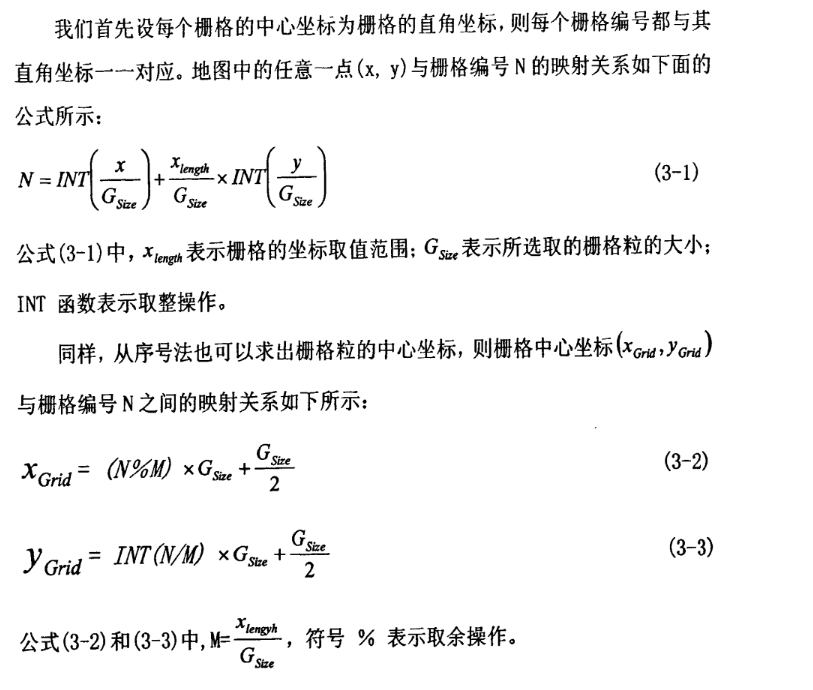
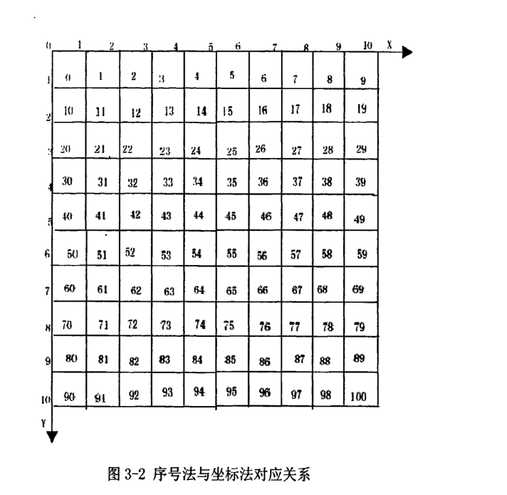
Modeling steps of indoor environment grid method

1. Selection of grid particle size

The size of the grid is a key factor. The selected grid is small, the environmental resolution is large, the storage of environmental information is large, and the decision-making speed is slow.

The grid selection is large, the environmental resolution is small, the storage of environmental information is small, and the decision-making speed is fast, but the ability to find paths in dense obstacle environment is weak.

2. Determination of obstacle grid

When the robot newly enters an environment, it does not know the information of indoor obstacles, which requires the robot to traverse the whole environment, detect the location of obstacles, find the serial number value in the corresponding grid map according to the location of obstacles, and modify the corresponding grid value. The free grid is assigned 0 to the grid without obstacles, and the obstacle grid is assigned 1 to the grid with obstacles

3. Establishment of grid map of unknown environment

The end point is usually set as an unreachable point, For example (- 1, - 1), at the same time, the robot follows the principle of "lower right, upper left" in the process of path finding, that is, the robot walks downward first. When the robot encounters an obstacle in front, the robot turns to the right. Following this rule, the robot can finally search all feasible paths, and the robot will eventually return to the starting point.

Note: on the grid map, there is a principle that the size of obstacles is always equal to the size of n grids, and half a grid will not appear.

3, Code

clc;
close all
clear
load('data1.mat')
S=(S_coo(2)-0.5)*num_shange+(S_coo(1)+0.5);%Number corresponding to the starting point
E=(E_coo(2)-0.5)*num_shange+(E_coo(1)+0.5);%Number corresponding to the end point

PopSize=20;%Population size
OldBestFitness=0;%Old optimal fitness value
gen=0;%Number of iterations
maxgen =100;%Maximum number of iterations

c1=0.6;%Wolf retention probability
c2=0.3;%Secondary wolf retention probability
c3=0.1;%Poor retention probability
%%
Alpha_score=inf; %change this to -inf for maximization problems
Beta_score=inf; %change this to -inf for maximization problems
Delta_score=inf; %change this to -inf for maximization problems
%Initialize the positions of search agents
%Initialization path
Group=ones(num_point,PopSize);  %Population initialization
flag=1;
%% Initialize particle swarm position


%Optimal solution
figure(1)
hold on
for i=1:num_shange
    for j=1:num_shange
        if sign(i,j)==1
            y=[i-1,i-1,i,i];
            x=[j-1,j,j,j-1];
            h=fill(x,y,'k');
            set(h,'facealpha',0.5)
        end
        s=(num2str((i-1)*num_shange+j));
        text(j-0.95,i-0.5,s,'fontsize',6)
    end
end
axis([0 num_shange 0 num_shange])%Boundary of restricted graph
plot(S_coo(2),S_coo(1), 'p','markersize', 10,'markerfacecolor','b','MarkerEdgeColor', 'm')%Draw starting point
plot(E_coo(2),E_coo(1),'o','markersize', 10,'markerfacecolor','g','MarkerEdgeColor', 'c')%Draw the end
set(gca,'YDir','reverse');%Image flip
for i=1:num_shange
    plot([0 num_shange],[i-1 i-1],'k-');
    plot([i i],[0 num_shange],'k-');%Draw grid lines
end
for i=2:index1
    Q1=[mod(route_lin(i-1)-1,num_shange)+1-0.5,ceil(route_lin(i-1)/num_shange)-0.5];
    Q2=[mod(route_lin(i)-1,num_shange)+1-0.5,ceil(route_lin(i)/num_shange)-0.5];
    plot([Q1(1),Q2(1)],[Q1(2),Q2(2)],'r','LineWidth',3)
end
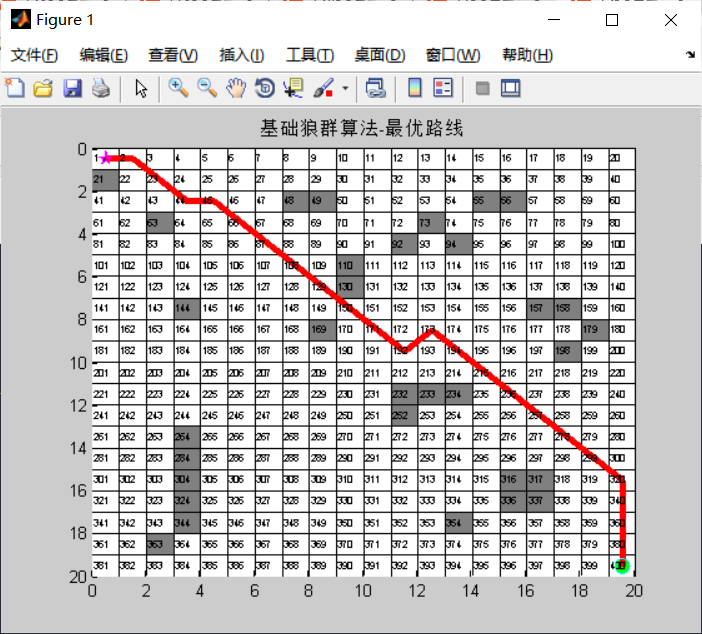
title('Basic wolf swarm algorithm-Optimal route');


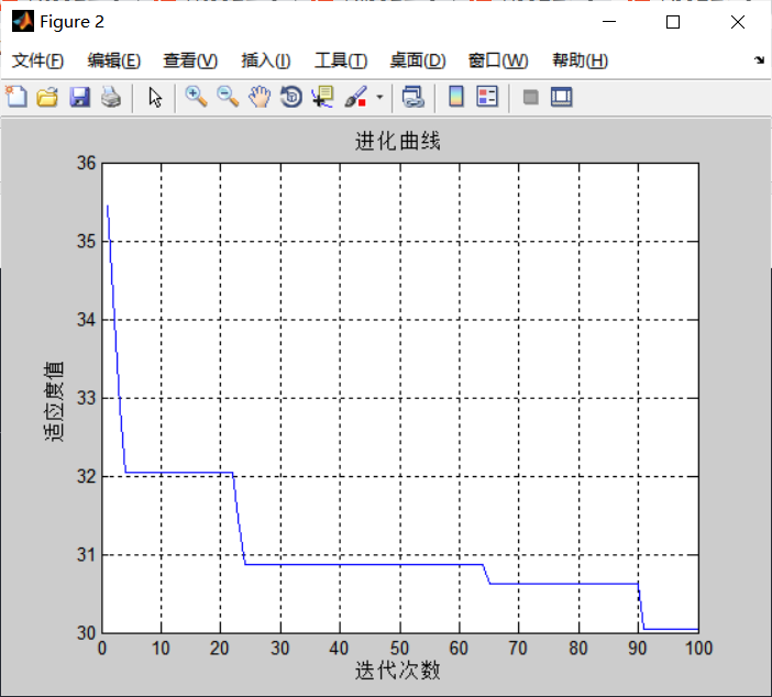
%Evolution curve
figure(2);
plot(BestFitness);
xlabel('Number of iterations')
ylabel('Fitness value')
grid on;
title('Evolution curve');
disp('Basic wolf swarm algorithm-Optimal route scheme:')
disp(num2str(route_lin))
disp(['Distance from start point to end point:',num2str(BestFitness(end))]);