With the continuous decline of the price of ngs, the transcriptome sequencing project has long entered the era of large samples. Of course, there was such a trend as early as the chip price was close to the people. At present, the price of single-cell transcriptome is also following this old path.

Then, for the transcriptome of large sample cohort, there is often no known reasonable grouping. At this time, it will be artificially grouped to see the heterogeneity of the cohort, such as grouping according to the level of immunity.

There are many ways to implement this grouping according to the immune level. Let's briefly demonstrate the hierarchical clustering of PCA and heat map and the scoring grouping such as gsea or gsva to see if there is any difference.

First look at the PCA grouping of the target gene set

Need to load step1 output The expression matrix in rdata file, oh, if you don't know step1 output Rdata if you get it, look at the code at the end of the text.

First, we need to advance the small expression matrix of immune gene set, and the code is as follows:

load(file = 'step1-output.Rdata')
cg=c('CD3D','CD3G CD247','IFNG','IL2RG','IRF1','IRF4','LCK','OAS2,STAT1')
cg
cg=cg[cg %in% rownames(dat)]
library("FactoMineR") #These two packages need to be loaded to draw the principal component analysis diagram
library("factoextra")  
dat.pca <- PCA(as.data.frame(t(dat[cg,]))  )
fviz_pca_ind(dat.pca,
             geom.ind = "point", # show points only (nbut not "text")
             # col.ind =  group_list, # color by groups 
             addEllipses = T,
             legend.title = "Groups"
)
dat.pca$ind$coord

As follows:

It can be seen that each sample has coordinates on this principal component analysis chart:

> head(dat.pca$ind$coord[,1:2])
                Dim.1      Dim.2
GSM1419942 -1.5307665  0.1820390
GSM1419943  0.2224343  0.9908672
GSM1419944 -2.1294537  0.3075360
GSM1419945  0.0745490  0.2147092
GSM1419946 -4.8646160 -0.2016098
GSM1419947  0.9149908  0.2421981

We can simply divide the sample into two groups according to PC1, or divide it into four groups according to PC1 and PC2. This step is very random. Let's try to divide the sample into two groups according to PC1. The code is as follows:

group_list=ifelse(dat.pca$ind$coord[,1] < 0 ,'neg','pos')
table(group_list) 
pca_gl = group_list
# Where hclust_gl comes from the previous tutorial
table(pca_gl,hclust_gl)

It can be seen that the sample grouping of the previous hierarchical clustering is still different from the grouping of PC1 of the current PCA:

> table(pca_gl,hclust_gl)
      hclust_gl
pca_gl high low
   neg    1  59
   pos   37  10

However, they are visually related, but there is not much difference:

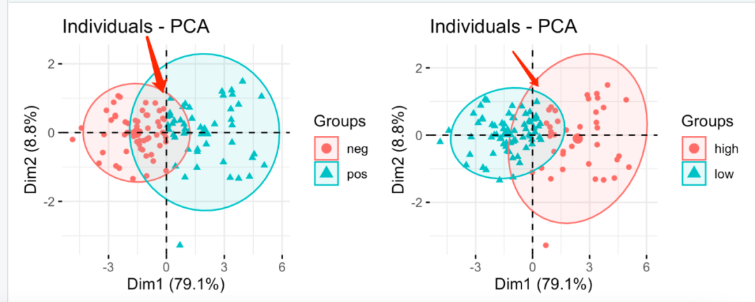
Differences between the two groups

The naked eye basically can't see the difference. The difference should be those samples near abscissa 0!

The code is:

library(patchwork)
fviz_pca_ind(dat.pca,
             geom.ind = "point", # show points only (nbut not "text")
             col.ind =  pca_gl, # color by groups 
             addEllipses = T,
             legend.title = "Groups"
)+ 
  fviz_pca_ind(dat.pca,
               geom.ind = "point", # show points only (nbut not "text")
               col.ind =  hclust_gl, # color by groups 
               addEllipses = T,
               legend.title = "Groups"
  )

It's very interesting. The samples with high and low immune classification in conflict between the two methods should have its special significance!

About step1 output Rdata this file

The above code loads step1 - output Rdata is a file. Here is how to make this file. The code is as follows:

rm(list = ls())  ## Magic operation, one key emptying~
options(stringsAsFactors = F)

library(AnnoProbe)
library(GEOquery) 
gset <- geoChina("GSE58812")
gset
gset[[1]]
a=gset[[1]] #
dat=exprs(a) #Now we need to know that expa is an object through the description of this function
dim(dat)#Look at the dimension of dat matrix
#   GPL570 [HG-U133_Plus_2] Affymetrix Human Genome U133 Plus 2.0 Array
dat[1:4,1:4] #Look at dat the 1 to 4 rows and 1 to 4 columns of this matrix. The row before the comma and the column after the comma
boxplot(dat[,1:4],las=2)  
dat=log2(dat)
boxplot(dat[,1:4],las=2)  
library(limma)
dat=normalizeBetweenArrays(dat)
boxplot(dat[,1:4],las=2)  
pd=pData(a) 
#By looking at the instruction manual, you can know to take the clinical information in object a and use pData
## Select some clinical phenotypes of interest.
library(stringr) 
table(pd$`meta:ch1`)
group_list= ifelse(pd$`meta:ch1` == '0' ,'stable','meta')
table(group_list)
 
dat[1:4,1:4]  
dim(dat)
a  
ids=idmap('GPL570','soft')
head(ids)
ids=ids[ids$symbol != '',]
dat=dat[rownames(dat) %in% ids$ID,]
ids=ids[match(rownames(dat),ids$ID),]
head(ids) 
colnames(ids)=c('probe_id','symbol')  
ids$probe_id=as.character(ids$probe_id)
rownames(dat)=ids$probe_id
dat[1:4,1:4] 

ids=ids[ids$probe_id %in%  rownames(dat),]
dat[1:4,1:4]   
dat=dat[ids$probe_id,] 

ids$median=apply(dat,1,median) #ids creates a new column called media. At the same time, it operates the dat matrix by row, takes the median of each row, and gives the result to each row of the column media
ids=ids[order(ids$symbol,ids$median,decreasing = T),]#Sort ids$symbol according to the order of ids$median from large to small, and assign the corresponding row as a new ids
ids=ids[!duplicated(ids$symbol),]#Take out the duplicate item from the symbol column, '!' If it is no, that is, take out the non duplicate items, remove the duplicate gene, and retain the maximum expression result of each gene s
dat=dat[ids$probe_id,] #Remove the probe from the new ids_ In the column ID, the dat is formed into a new dat according to each row in the extracted column
rownames(dat)=ids$symbol#Give each row in the symbol column of ids to dat as the row name of dat
dat[1:4,1:4]  #Keep the information of the first occurrence of each gene ID

dat['ACTB',]
dat['GAPDH',]
save(dat,group_list,
     file = 'step1-output.Rdata')

If you really think my tutorial is helpful to your scientific research project and makes you enlightened, or your project uses a lot of my skills, please add a short thank you when publishing your achievements in the future, as shown below:

We thank Dr.Jianming Zeng(University of Macau), and all the members of his bioinformatics team, biotrainee, for generously sharing their experience and codes.

If I have traveled around the world in universities and research institutes (including Chinese mainland) in ten years, I will give priority to seeing you if you have such a friendship.