According to Forbes, about 2.5 million bytes of data are generated every day. These data can then be analyzed using data science and machine learning techniques to provide analysis and prediction. Although in most cases, the initially collected data needs to be preprocessed before starting any statistical analysis. There are many different reasons for the need for pretreatment analysis, such as:
- The collected data format is incorrect (such as SQL database, JSON, CSV, etc.)
- Missing and outliers
- Standardization
- Reduce the inherent noise in the data set (some stored data may be damaged)
- Some features in the dataset may not be able to collect any information for analysis
In this article, I will show you how to use python to reduce the number of features in the kaggle Mushroom Classification dataset.
Reducing the number of features to be used during statistical analysis may bring some benefits, such as:
- Improve accuracy
- Reduce the risk of overfitting
- Speed up your training
- Improve data visualization
- Increase the interpretability of our model
In fact, it is statistically proved that when performing machine learning tasks, there are the best number of features that should be used for each specific task (Fig. 1). If more features are added than necessary, the performance of our model will degrade (because noise is added). The real challenge is to find out which features are the best use features (which actually depends on the amount of data we provide and the complexity of the task we are trying to achieve). This is where feature selection technology can help us!
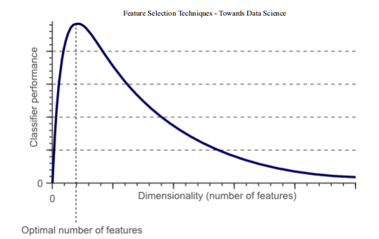
Figure 1: relationship between classifier performance and dimensions
feature selection
There are many different methods for feature selection. The most important of these are:
1. Filtering method = filter our data set and only take the subset containing all relevant features (for example, use Pearson correlation matrix).
2. Follow the same objectives of the filtering method, but use the machine learning model as its evaluation criteria (e.g., forward / backward / bidirectional / recursive feature elimination). We input some features into the machine learning model, evaluate their performance, and then decide whether to add or delete features to improve accuracy. Therefore, this method can be more accurate than filtering, but the computational cost is higher.
3. Embedding method. Like the filtering method, the embedding method also uses the machine learning model. The difference between the two methods is that the embedded method checks the different training iterations of ML model, and then sorts the importance of each feature according to the contribution of each feature to ML model training.
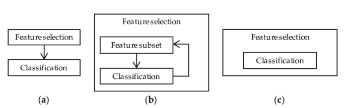
Figure 2: representation of filters, wrappers and embedded methods [3]
practice
In this article, I will use the Mushroom Classification dataset to try to predict whether mushrooms are poisonous by looking at a given characteristic. While doing so, we will try different feature elimination techniques to see how they affect the training time and the overall accuracy of the model.
Data download: https://github.com/ffzs/dataset/blob/master/mushrooms.csv
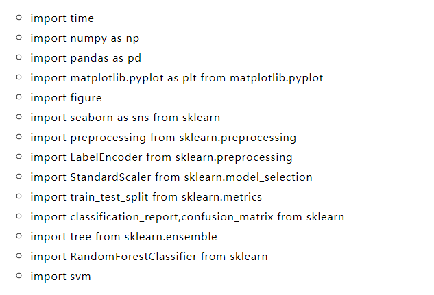
First, we need to import all the necessary libraries.
The dataset we will use in this example is shown in the following figure.

Figure 3: Mushroom Classification dataset
Before inputting these data into the machine learning model, I decided to conduct one hot coding for all classification variables, divide the data into feature (x) and label (y), and finally conduct it in the training set and test set.
X = df.drop(['class'], axis = 1)
Y = df['class']
X = pd.get_dummies(X, prefix_sep='_')
Y = LabelEncoder().fit_transform(Y)

X2 = StandardScaler().fit_transform(X)

X_Train, X_Test, Y_Train, Y_Test = train_test_split(X2, Y, test_size = 0.30,  random_state = 101)
Characteristic importance
Set based decision tree model (such as random forest) can be used to rank the importance of different features. Understanding the most important features of our model is crucial to understanding how our model makes predictions (making them easier to interpret). At the same time, we can remove features that are not good for our model.
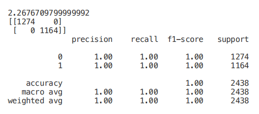
start = time.process_time()
trainedforest = RandomForestClassifier(n_estimators=700).fit(X_Train,Y_Train)
print(time.process_time() - start)
predictionforest = trainedforest.predict(X_Test)
print(confusion_matrix(Y_Test,predictionforest))
print(classification_report(Y_Test,predictionforest))
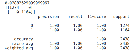
As shown in the figure below, a random forest classifier is trained with all features, and 100% accuracy is obtained in about 2.2 seconds. In each example below, the training time of each model will be printed on the first line of each segment for your reference.
Once our random forest classifier is trained, we can create a feature importance graph to see which features are most important for our model prediction (Figure 4). In this example, only the first seven features are shown below.
figure(num=None, figsize=(20, 22), dpi=80, facecolor='w', edgecolor='k')

feat_importances = pd.Series(trainedforest.feature_importances_, index= X.columns)
feat_importances.nlargest(7).plot(kind='barh')
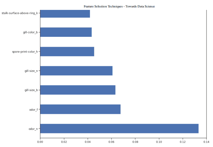
Figure 4: feature importance diagram
Now that we know which features are considered most important by our random forest, we can try to use the first three to train our model.
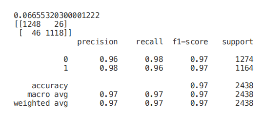
X_Reduced = X[['odor_n','odor_f', 'gill-size_n','gill-size_b']]
X_Reduced = StandardScaler().fit_transform(X_Reduced)
X_Train2, X_Test2, Y_Train2, Y_Test2 = train_test_split(X_Reduced, Y, test_size = 0.30,  random_state = 101)

start = time.process_time()
trainedforest = RandomForestClassifier(n_estimators=700).fit(X_Train2,Y_Train2)
print(time.process_time() - start)
predictionforest = trainedforest.predict(X_Test2)
print(confusion_matrix(Y_Test2,predictionforest))
print(classification_report(Y_Test2,predictionforest))
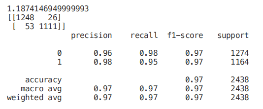
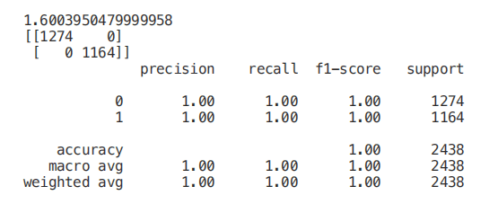
As we can see below, using only three features will only reduce the accuracy by 0.03% and reduce the training time by half.
We can also understand how to make feature selection by visualizing a trained decision tree.
start = time.process_time()
trainedtree = tree.DecisionTreeClassifier().fit(X_Train, Y_Train)
print(time.process_time() - start)
predictionstree = trainedtree.predict(X_Test)
print(confusion_matrix(Y_Test,predictionstree))
print(classification_report(Y_Test,predictionstree))
The features at the top of the tree structure are the most important features that our model retains in order to perform classification. Therefore, selecting only the first few features at the top and abandoning other features may create a model with considerable accuracy.
import graphviz
from sklearn.tree import DecisionTreeClassifier, export_graphviz


data = export_graphviz(trainedtree,out_file=None,feature_names= X.columns,
        class_names=['edible', 'poisonous'],
        filled=True, rounded=True,
        max_depth=2,
        special_characters=True)
graph = graphviz.Source(data)
graph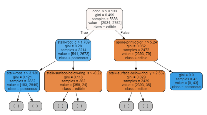
Figure 5: Decision Tree Visualization
Recursive feature elimination (RFE)
Recursive feature elimination (RFE) takes the instance of machine learning model and the final expected number of features to be used as input. Then, it recursively reduces the number of features to be used by ranking them using machine learning model accuracy as a measure.
Create a for loop in which the number of input features is our variable, so that we can find the best number of features required by our model by tracking the accuracy registered in each loop iteration. Using the RFE support method, we can find the name of the feature evaluated as the most important (rfe.support returns a Boolean list, where true indicates that a feature is considered important and false indicates that a feature is not important).
from sklearn.feature_selection import RFE

model = RandomForestClassifier(n_estimators=700)
rfe = RFE(model, 4)
start = time.process_time()
RFE_X_Train = rfe.fit_transform(X_Train,Y_Train)
RFE_X_Test = rfe.transform(X_Test)
rfe = rfe.fit(RFE_X_Train,Y_Train)
print(time.process_time() - start)
print("Overall Accuracy using RFE: ", rfe.score(RFE_X_Test,Y_Test))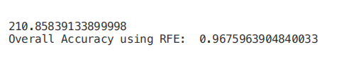
SelecFromModel
Select from model is another scikit learning method, which can be used for feature selection. This method can be used for all different types of scikit learning models with coef or feature importance attributes (after fitting). Select from model is a less reliable solution than rfe. In fact, select from model just deletes less important features based on the calculated threshold (which does not involve the optimization iteration process).
To test the validity of select from model, I decided to use an extratrees classifier in this example.
Extreesclassifier (extreme random tree) is a tree based integrated classifier. Compared with random forest method, it can produce less variance (thus reducing the risk of over fitting). The main difference between random forest and extremely random tree is that the sampling of nodes in extremely random tree does not need to be replaced.
from sklearn.ensemble import ExtraTreesClassifier
from sklearn.feature_selection import SelectFromModel

model = ExtraTreesClassifier()
start = time.process_time()
model = model.fit(X_Train,Y_Train)
model = SelectFromModel(model, prefit=True)
print(time.process_time() - start)
Selected_X = model.transform(X_Train)

start = time.process_time()
trainedforest = RandomForestClassifier(n_estimators=700).fit(Selected_X, Y_Train)
print(time.process_time() - start)
Selected_X_Test = model.transform(X_Test)
predictionforest = trainedforest.predict(Selected_X_Test)
print(confusion_matrix(Y_Test,predictionforest))
print(classification_report(Y_Test,predictionforest))
Correlation matrix analysis
In order to reduce the number of features in the dataset, another possible method is to check the correlation between features and labels.
Using Pearson correlation, our return coefficient value will vary between - 1 and 1:
- If the correlation between two features is 0, it means that changing either feature will not affect the other.
- If the correlation between two features is greater than 0, it means that increasing the value in one feature will also increase the value in another feature (the closer the correlation coefficient is to 1, the stronger the relationship between two different features).
- If the correlation between two features is less than 0, it means that increasing the value in one feature will reduce the value in the other feature (the closer the correlation coefficient is to - 1, the stronger the relationship between two different features).
In this case, we will only consider the characteristics related to the output variable of at least 0.5.
Numeric_df = pd.DataFrame(X)
Numeric_df['Y'] = Y
corr= Numeric_df.corr()
corr_y = abs(corr["Y"])
highest_corr = corr_y[corr_y >0.5]
highest_corr.sort_values(ascending=True)

We can now study the relationship between different correlation features more carefully by creating a correlation matrix.
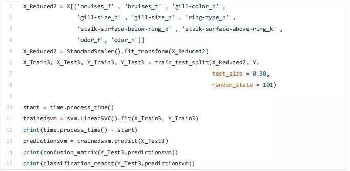
figure(num=None, figsize=(12, 10), dpi=80, facecolor='w', edgecolor='k')

corr2 = Numeric_df[['bruises_f' , 'bruises_t' , 'gill-color_b' , 'gill-size_b' ,  'gill-size_n' , 'ring-type_p' , 'stalk-surface-below-ring_k' ,  'stalk-surface-above-ring_k' , 'odor_f', 'odor_n']].corr()

sns.heatmap(corr2, annot=True, fmt=".2g")
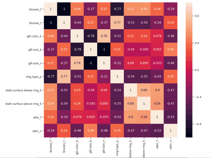
Figure 6: correlation matrix of the highest correlation feature
Another aspect that may be controlled in this analysis is to check whether the selected variables are highly correlated with each other. If so, we just need to keep one of them and remove the others.
Finally, we can now select only the features with the highest correlation with y and train / test a support vector machine model to evaluate the results of this method.
Univariate selection
Univariate feature selection is a statistical method used to select the features most closely related to our corresponding tags. Using the selectkbest method, we can decide which metrics to use to evaluate our features and the number of k best features we want to keep. According to our needs, different types of scoring functions are provided:
- Classification = chi2, f_classif, mutual_info_classif
- Regression = f_regression, mutual_info_regression
In this example, we will use chi2 (Figure 7).
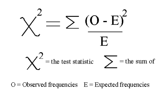
Figure 7: Chi square formula [4]
Chi squared (chi2) can take non negative values as input, so first, we scale the input data between 0 and 1.
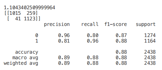
from sklearn.feature_selection import SelectKBest
from sklearn.feature_selection import chi2

min_max_scaler = preprocessing.MinMaxScaler()
Scaled_X = min_max_scaler.fit_transform(X2)

X_new = SelectKBest(chi2, k=2).fit_transform(Scaled_X, Y)
X_Train3, X_Test3, Y_Train3, Y_Test3 = train_test_split(X_new, Y, test_size = 0.30,  random_state = 101)
start = time.process_time()
trainedforest = RandomForestClassifier(n_estimators=700).fit(X_Train3,Y_Train3)
print(time.process_time() - start)
predictionforest = trainedforest.predict(X_Test3)
print(confusion_matrix(Y_Test3,predictionforest))
print(classification_report(Y_Test3,predictionforest))
Lasso Regression
When applying regularization to machine learning model, we add a penalty to the model parameters to avoid our model trying to get too close to our input data. In this way, we can make our model less complex, and we can avoid over fitting (so that our model can learn not only the key data features, but also its internal noise).
One possible regularization method is lasso regression. When lasso regression is used, if the coefficients of input features do not make a positive contribution to our machine learning model training, they will shrink. In this way, some features may be automatically discarded, i.e. their coefficients are specified as zero.
from sklearn.linear_model import LassoCV

regr = LassoCV(cv=5, random_state=101)
regr.fit(X_Train,Y_Train)
print("LassoCV Best Alpha Scored: ", regr.alpha_)
print("LassoCV Model Accuracy: ", regr.score(X_Test, Y_Test))
model_coef = pd.Series(regr.coef_, index = list(X.columns[:-1]))
print("Variables Eliminated: ", str(sum(model_coef == 0)))
print("Variables Kept: ", str(sum(model_coef != 0)))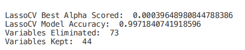
Once our model is trained, we can create a feature importance graph again to understand which features are considered most important by our model (Figure 8). This is very useful, especially when trying to understand how our model decides to make predictions, so it makes our model easier to explain.
figure(num=None, figsize=(12, 10), dpi=80, facecolor='w', edgecolor='k')

top_coef = model_coef.sort_values()
top_coef[top_coef != 0].plot(kind = "barh")
plt.title("Most Important Features Identified using Lasso (!0)")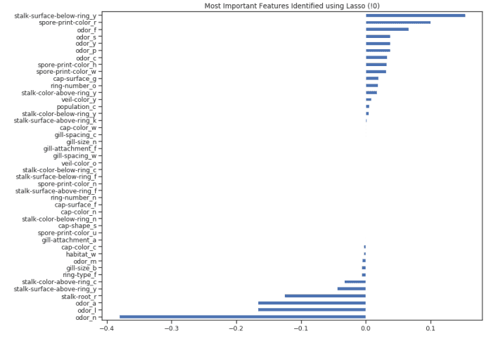
Figure 8: lasso feature importance diagram
Source: https://towardsdatascience.com/feature-selection-techniques-1bfab5fe0784