Creating a bitcoin trading robot will not lose money
In this article, we will create a deep reinforcement learning agent to learn to make money through bitcoin trading. In this tutorial, we will use the PPO agent in OpenAIgym and the stable baselines Library (a branch of OpenAI's baselines Library).
The purpose of this series of articles is to try Ť h state of the art deep reinforcement learning technology to see if we can create profitable bitcoin trading robots. Any attempt to quickly stop creating reinforcement learning algorithms seems to be the status quo because it is "the wrong way to build trading algorithms". However, the latest progress in this field shows that RL agents usually have much better learning ability than supervised learning agents in the same problem domain. For this reason, I write these articles to see how much money we can make these trading agents, or whether there is a current situation for some reason.
Many thanks to OpenAI and DeepMind for the open source software they have been providing to deep learning researchers for the past two years. If you haven't seen their amazing achievements using technologies such as AlphaGo, OpenAI Five and AlphaStar, you may have been living in trouble for the past year, but you should also see them.
Although we will not create anything impressive, it is still not easy to realize the profitable trading of bitcoin on a daily basis. this paper
1. Create a learning fitness environment for our agents
2. Presents a simple and elegant visualization of the environment
3. Train our agents to learn profitable trading strategies
If you are not familiar with how to create a fitness environment from scratch, or how to present these Simple visualization of environment Well, I just wrote an article on these two topics. Pause here at any time and read any of them before continuing.
introduction
In this tutorial, we will use the Kaggle dataset generated by Zielak. If you want to download the code to continue csv, which will also be available in my GitHub repository. Well, let's start.
First, let's import all the necessary libraries. Make sure pip install you are missing any libraries
import gym
import pandas as pd
import numpy as np
from gym import spaces
from sklearn import preprocessing
Next, let's create our classes for the environment. We will need pandas to pass in a data frame and an optional initial_balance, and a lookback_window_size to indicate how many time steps the agent will observe at each step in the past. We will set the default price of each transaction of the commission to 0.075% of the current Bitmex exchange rate, and set the default value of the serial parameter to false, which means that by default, our data frames will be traversed randomly.
We also call dropna() and reset on the data frame_ Index(), first delete all rows with NaN value, and then reset the index of the frame because the data is deleted.
class BitcoinTradingEnv(gym.Env):
  """A Bitcoin trading environment for OpenAI gym"""
  metadata = {'render.modes': ['live', 'file', 'none']}
  scaler = preprocessing.MinMaxScaler()
  viewer = None
  def __init__(self, df, lookback_window_size=50,
                         commission=0.00075,
                         initial_balance=10000
                         serial=False):
    super(BitcoinTradingEnv, self).__init__()
    self.df = df.dropna().reset_index()
    self.lookback_window_size = lookback_window_size
    self.initial_balance = initial_balance
    self.commission = commission
    self.serial = serial
  # Actions of the format Buy 1/10, Sell 3/10, Hold, etc.
    self.action_space = spaces.MultiDiscrete([3, 10])
  # Observes the OHCLV values, net worth, and trade history
    self.observation_space = spaces.Box(low=0, high=1, shape=(10,
                    lookback_window_size + 1), dtype=np.float16)
Our action_space is represented here as a set of discrete 3 options (buy, sell or hold) and another set of discrete 10 quantities (1/10, 2/10, 3/10, etc). After selecting the purchase action, we will purchase amount * self Balance value BTC. For selling behavior, we will sell amount * self btc_ Hold value BTC. Of course, the hold operation ignores the amount and does nothing.
We observe_ Space is defined as a continuous floating-point set between 0 and 1, and its shape is * * (10, lookback_window_size + 1). The + 1 is to consider the current time step. For each time step in the window, we will observe the OHCLV * * (open, high, close, low, volume) value, our net worth, the number of BTCs purchased or sold, and the total amount of dollars we spend on or get from these BTCs.
Next, we need to write our reset method to initialize the environment.
def reset(self):
  self.balance = self.initial_balance
  self.net_worth = self.initial_balance
  self.btc_held = 0
  self._reset_session()
  self.account_history = np.repeat([
    [self.net_worth],
    [0],
    [0],
    [0],
    [0]
  ], self.lookback_window_size + 1, axis=1)
  self.trades = []
  return self._next_observation()
Here, we also use self_ reset_ Session and self_ next_ Observation, we haven't defined it yet. Let's define them.
1. Trading period
The concept of trade conference is an important part of our environment. If we want to deploy the agent in the field, we may never run for more than two months. Therefore, we will limit self The number of consecutive frames that the DF proxy sees in succession.
In our_ reset_ In the session method, we will first reset current_step is 0. Next, we will set steps_left a random number between 1 and MAX_TRADING_SESSION, which will now be defined at the top of the file.
MAX_TRADING_SESSION = 100000#〜2 Months
Next, if you want to traverse the frame serially, set the entire frame to be traversed to no, otherwise set it to frame_ Random point self in start DF and create a new data frame called active_df, the data frame is only self dffromframe_ Part of the frame from start to to_ start + steps_ left.
def _reset_session(self):
  self.current_step = 0
  if self.serial:
    self.steps_left = len(self.df) - self.lookback_window_size - 1
    self.frame_start = self.lookback_window_size
  else:
    self.steps_left = np.random.randint(1, MAX_TRADING_SESSION)
    self.frame_start = np.random.randint(
         self.lookback_window_size, len(self.df) - self.steps_left)
  self.active_df = self.df[self.frame_start -
       self.lookback_window_size:self.frame_start + self.steps_left]
An important side effect of traversing data frames in random slices is that after a long time of training, our agent will have more unique data to process. For example, if we only traverse the data frame serially (i.e. from 0 to len(df)), we will only have as many unique data points as in the data frame. Our observation space can even show a discrete number of states in each time step.
However, by randomly traversing the segments of the data frame, we can create more unique data points by creating more interesting account balances for each time step in the initial data set, the combination of closed transactions and previously seen price behavior. Let me explain with an example.
In step 10 after resetting the serial environment, our agent will always be at the same time in the data frame, and there are three options at each time step: buy, sell or hold. For each of these three options, another option will be required: 10%, 20%,... Or 100% of the possible quantity. This means that our agent may experience (1 ³³)¹ ⁰ any of the total States, there may be 1 ⁰ in total ³ A unique experience.
Now consider our random slicing environment. At time step 10, our agent can at any time step within the len(df) data frame. Given the same choice for each time step, this means that the agent can len(df) experience any change in the same 10 time steps ³ ⁰ one possible unique state.
Although this may add a lot of interference to large data sets, I think it should allow agents to learn more from our limited data. We will still traverse our test data set serially to more accurately understand the usefulness of the algorithm for fresh, seemingly "real-time" data.
Life Through The Agent's Eyes
Below it is the trading volume, while below it is a strange Morse code, such as the interface showing the trading history. It seems that our agent should be able to fully learn observation from our data_ Space, so let's continue. Here, we will define_ next_ The observation method scales the observed data to a range from 0 to 1.
def _next_observation(self):
  end = self.current_step + self.lookback_window_size + 1
  obs = np.array([
    self.active_df['Open'].values[self.current_step:end],
    self.active_df['High'].values[self.current_step:end],
    self.active_df['Low'].values[self.current_step:end],
    self.active_df['Close'].values[self.current_step:end],
    self.active_df['Volume_(BTC)'].values[self.current_step:end],
  ])
  scaled_history = self.scaler.fit_transform(self.account_history)
  obs = np.append(obs, scaled_history[:, -(self.lookback_window_size
                                                     + 1):], axis=0)
  return obs
Taking Action
Now that we have established the observation space, it's time to write the step function and take the specified actions of the agent. self.steps_left == 0 at any time during the current trading period, we will sell any BTC we hold and send it to**_ reset_session()**. Otherwise, we will set reward to the current net assets, and set done to True only when the funds are exhausted.
def step(self, action):
  current_price = self._get_current_price() + 0.01
  self._take_action(action, current_price)
  self.steps_left -= 1
  self.current_step += 1
  if self.steps_left == 0:
    self.balance += self.btc_held * current_price
    self.btc_held = 0
    self._reset_session()
  obs = self._next_observation()
  reward = self.net_worth
  done = self.net_worth <= 0
  return obs, reward, done, {}
Take action and get current first_ Price is as simple as determining a specified action and buying and selling a specified number of BTC s. Let's write it quickly_ take_action so that we can test our environment.
Finally, using the same method, we will append the transaction to self Trade and update our net assets and account history.
def _take_action(self, action, current_price):
  action_type = action[0]
  amount = action[1] / 10
  btc_bought = 0
  btc_sold = 0
  cost = 0
  sales = 0
  if action_type < 1:
    btc_bought = self.balance / current_price * amount
    cost = btc_bought * current_price * (1 + self.commission)
    self.btc_held += btc_bought
    self.balance -= cost
  elif action_type < 2:
    btc_sold = self.btc_held * amount
    sales = btc_sold * current_price  * (1 - self.commission)
    self.btc_held -= btc_sold
    self.balance += sales

  if btc_sold > 0 or btc_bought > 0:
	  self.trades.append({
	     'step': self.frame_start+self.current_step,
	     'amount': btc_sold if btc_sold > 0 else btc_bought,
	     'total': sales if btc_sold > 0 else cost,
	     'type': "sell" if btc_sold > 0 else "buy"
	   })
	 self.net_worth = self.balance + self.btc_held * current_price
	 self.account_history = np.append(self.account_history, [
	   [self.net_worth],
	   [btc_bought],
	   [cost],
	   [btc_sold],
	   [sales]
	 ], axis=1)
Our agents can now start a new environment, step through the environment and take actions that affect the environment. It's time to see them trade.
Watch our robot deal
Our render method may be as simple as calling print(self.net_worth), but it's no fun. Instead, we will draw a simple candlestick chart of price data with quantity bars and a separate chart for our net worth.
We stocktradinggraph Py will be from Last article Get the code and repurpose it to render our bitcoin environment. You can get it from my GitHub Get code on.
The first change we want to make is to update all locations to self DF ['Date'] is self DF ['Timestamp'], and delete all calls to date2num, because our Date has adopted Unix Timestamp format. Next, in our render method, we will update the Date tag to print a human readable Date instead of a number.
from datetime import datetime
First, import the datetime library, then use the utcfromtimestamp method to get the UTC string from each timestamp, and strftime format the string Y-m-d H:M in format.
date_labels = np.array([datetime.utcfromtimestamp(x).strftime(
'%Y-%m-%d %H:%M') for x in self.df['Timestamp'].values[step_range]])
Finally, we make the change self DF ['Volume'] with self DF ['Volume_5; (BTC)'] matches our dataset and we're doing well. Back to BitcoinTradingEnv, we can now write our render method to display graphics.
def render(self, mode='human', **kwargs):
  if mode == 'human':
    if self.viewer == None:
      self.viewer = BitcoinTradingGraph(self.df,
                                        kwargs.get('title', None))
    self.viewer.render(self.frame_start + self.current_step,
                       self.net_worth,
                       self.trades,
                       window_size=self.lookback_window_size)
Look! Now, we can see our agents trading bitcoin.
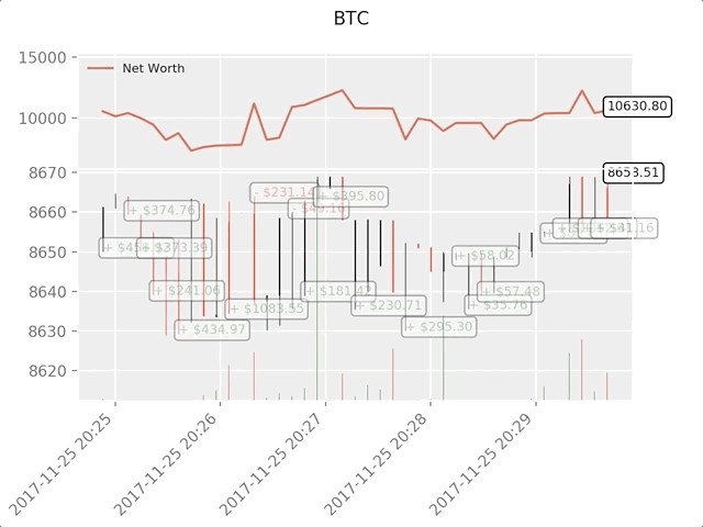
The green phantom label represents the purchase of BTC, and the red phantom label represents the sale of BTC. The white label in the upper right corner is the agent's current net asset value, and the label in the lower right corner is the current price of bitcoin. Simple and elegant. Now, it's time to train our agents and see how much money we can make!
training time
One of the criticisms I received in the first article was the lack of cross validation or the failure to divide the data into training sets and test sets. The purpose of this is to test the accuracy of the final model based on new data that has never been available. Although this is not the focus of this article, it is definitely here. Because we use time series data, we don't have much choice in cross validation.
For example, a common form of cross validation is called k-fold validation, in which you divide the data into k equal groups, and then use them as test groups one by one, and the rest of the data as training groups. However, time series data are highly time-dependent, which means that future data are highly dependent on previous data. Therefore, the k-discount does not work because our brokers will learn from future data before they have to trade, which is an unfair advantage.
This same flaw applies to most other cross validation strategies when applied to time series data. Therefore, we only need to take a slice of the whole data frame from the beginning of the frame to an arbitrary index as the training set, and then use the rest of the data as the test set.
slice_point = int(len(df) - 100000)
train_df = df[:slice_point]
test_df = df[slice_point:]
Now I divide our data frame into training set and data set
train_env = DummyVecEnv([lambda: BitcoinTradingEnv(train_df,
                         commission=0, serial=False)])
test_env = DummyVecEnv([lambda: BitcoinTradingEnv(test_df,
                        commission=0, serial=True)])
Next, we train our model in the interaction between agent and environment
model = PPO2(MlpPolicy,
             train_env,
             verbose=1,
             tensorboard_log="./tensorboard/")
model.learn(total_timesteps=50000)
Here, we are using tensorboard, so we can easily visualize the tensor flow graph and see some quantitative indicators about agents. For example, the following is a chart of post discount rewards for many agents over 200000 time steps:
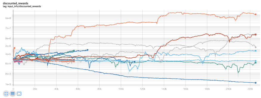
Wow, it seems that our agent is very profitable! Our best brokers can even increase their balance by 1000 times in 200000 steps, and the rest by at least 30 times on average! It is at this point that I realize that there is an error in the environment... This is the new reward map after fixing the error:
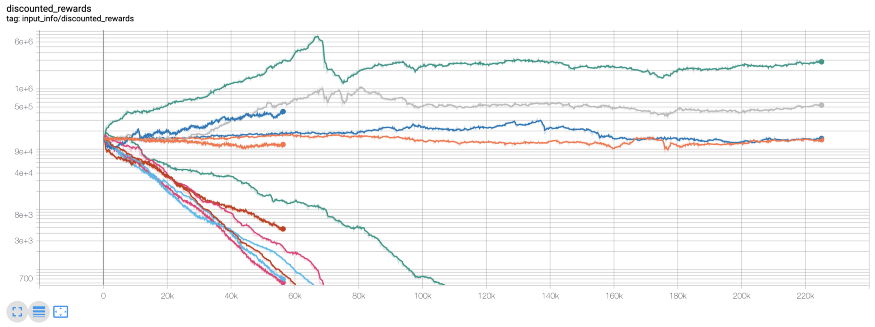
As you can see, several of our agents are doing well, and the rest are bankrupt. However, agents with excellent performance can only increase their initial balance by 10 times or even 60 times at most. I must admit that all profitable agents are trained and tested without commission. Therefore, it is unrealistic for our agents to make money. But we're somewhere!
Let's test our agents in a test environment (using fresh data they've never seen) to see how they learn to trade bitcoin.
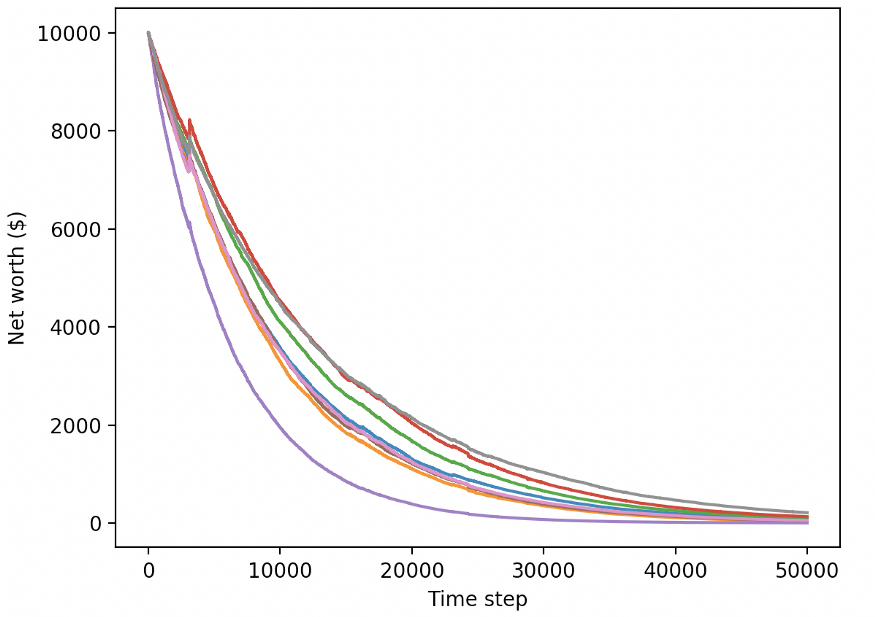
Obviously, we still have a lot of work to do. By simply switching the model to A2C using a stable benchmark (instead of the current PPO2 agent), we can greatly improve the performance of this dataset. Finally, according to Sean O'Gorman's suggestion, we can slightly update the reward function so that we can reward increased net assets, not just get higher net assets and stay there.
reward = self.net_worth - prev_net_worth
These two changes alone can greatly improve the performance of the test data set, and as you can see below, we can finally make a profit from the fresh data not available in the training set.
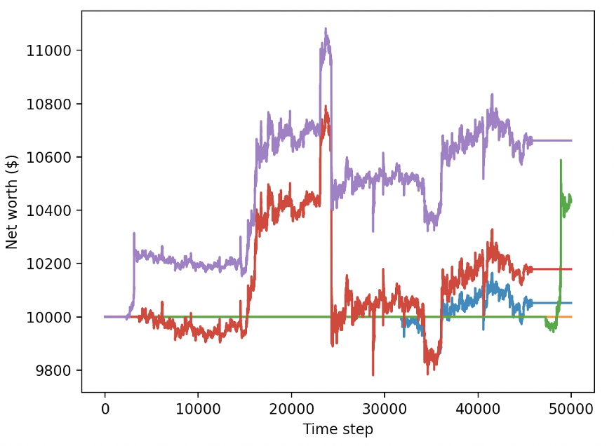
However, we can do better. In order to improve these results, we will need to optimize our super parameters and train our agents for a longer time. It's time to break the GPU and start working!
However, this article is a little long, and we still have a lot of details to discuss, so we will take a break here. In my next article, we will use Bayesian optimization to allocate the best super parameters for our problem space and improve the agent's model to achieve a high-profit trading strategy.
conclusion
In this paper, we begin to use deep reinforcement learning to create a profitable bitcoin trading agent from scratch. We can accomplish the following tasks:
A bitcoin trading environment was created from scratch using OpenAI's gym.
The visualization of the environment is built using Matplotlib.
Use simple cross validation to train and test our agents.
Slightly adjust our agents to achieve profitability.
Although the profits of our trading agency are not as good as we hope, it is certainly making progress. Next time, we will improve these algorithms through advanced functional engineering and Bayesian optimization to ensure that our agents can consistently beat the market. Please continue to follow my Next article, long live bitcoin!
reference: https://towardsdatascience.com/creating-bitcoin-trading-bots-that-dont-lose-money-2e7165fb0b29