Timing analysis 26

Preliminary study on time series prediction Prophet package

preface

In the previous articles in this series, we introduced a variety of time series prediction techniques and models. We can see that the time series prediction technology is still very complex and the steps are cumbersome. Readers may remember that VAR model has many steps and involves many knowledge points and concepts.

This article will introduce the Facebook open source timing prediction package prophet Prophet's designers believe that time series prediction should be simple and easy to use for those who analyze and use the technology, without going through all the popular standard methods. Prophet was born on the basis of the original intention of this design.

We will use Prophet's method to predict the effect of VAR in this paper. The example used is a financial problem. We hope to predict the monthly net sales of hypothetical food and beverage companies in a country from April to December 2020, and dig out the growth and losses in an uncertain economic environment. Some assumptions are made: an enterprise with complex supply chain network needs domestic and foreign raw material supply at the same time; And the customer channels are also diverse, including domestic channels and global channels. Therefore, the company will be very affected by customer emotion, retail industry, industrial production and supply chain. In other words, the company as a whole is very sensitive to procurement, production and distribution, both domestically and globally.

Time series prediction problem

Firstly, time series prediction is a very complex problem, but it is of great significance. The most common question is about sales. Enterprise data scientists, business analysts and managers all want to measure potential growth, the possibility of loss and uncertainty in some difficult times. In addition, time series forecasting has strong demand in weather, stock market, macro-economy (GDP), e-commerce, retail and other fields.

Secondly, it is very difficult to predict the future. Although there are many methods of time series prediction, such as ARIMA (see another article of the author) Time series analysis (6) – ARIMA(p,d,q) model ), SARIMA and LSTM, which are popular in recent years, have obvious disadvantages. We know that the first two methods are more suitable for univariate time series prediction; LSTM is a black box method with low interpretability. In this article, we will introduce Prophet package in the way of combining theory with practice, and compare VAR model (see another article of the author) Time series analysis (19 vector autoregressive (VAR)) The prediction effect of article and Prophet.
Thirdly, VAR is a multivariable regression model, which can predict multiple time series at the same time; Prophet is a univariate prediction, but it has the ability to add additional factors.

Finally, the author understands that the prediction problems based on data science are the historical characteristics and laws of mining data, which will appear in the future, which is the underlying logic that prediction can become possible. If new features and laws appear or the old model has failed, the prediction is impossible to be accurate.

Prophet basic mode

Prophet is based on the general additive model (GAM).
y ( t ) = g ( t ) + s ( t ) + h ( t ) + ϵ t {\LARGE y(t)=g(t)+s(t)+h(t)+\epsilon_t } y(t)=g(t)+s(t)+h(t)+ϵt​

• g ( t ) g(t) g(t) represents the trend function
• s ( t ) s(t) s(t) represents seasonal or periodic changes, such as weekly and annual
• h ( t ) h(t) h(t) represents holiday factors
  and ϵ t \epsilon_t ϵ t ， is the error term not captured by the model.

Prophet considers trend factors and cyclical factors, which are very many patterns in retail, economy and finance, and holiday factors usually affect the fluctuation of time series. Prophet's basic idea still focuses on the components of the practice sequence, such as frequency, periodicity, trend and domain knowledge, and the last point is very important.

1. Import package

import pandas as pd
import numpy as np

import matplotlib.pyplot as plt
import matplotlib as mpl
mpl.rcParams['figure.figsize'] = 16, 10
import seaborn as sns
sns.set_style('ticks')
%matplotlib inline

from fbprophet import Prophet
from fbprophet.diagnostics import cross_validation

import statsmodels.api as sm
from statsmodels.tsa.api import VAR
import matplotlib.pyplot as plt
from statsmodels.tsa.stattools import adfuller
from statsmodels.tools.eval_measures import rmse, aic


import os
from IPython.display import HTML

2. Read in the data and clean the data

### disable scientific notation in pandas
pd.set_option('display.float_format', '{:.2f}'.format) ### isplay up to 2 decimal pts

salesdf = pd.read_csv('E:\datasets\salesdf.csv')
salesdf ['Date'] = pd.DatetimeIndex(salesdf ['Date'])

pd.set_option('display.max_rows', 10)
salesdf.head()

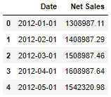
The above figures are hypothetical data on net sales in Germany

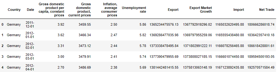
The following macroeconomic index data, such as unit capital, GDP, consumer price, average inflation and unemployment rate, are derived from the IMF, https://www.imf.org/external/pubs/ft/weo/2020/01/weodata/index.aspx
The import and export data comes from OECD, https://data.oecd.org/trade/trade-in-goods-and-services-forecast.htm

all_indicators = pd.read_csv('E:\datasets\economic_indicator_yearly.csv')

### Interpolate the data monthly
### Specifically, we change the frequency from yearly to monthly and interpolate the missing data using linear intepolation

all_indicators['Date'] = pd.DatetimeIndex(all_indicators['Date'])
all_indicators = all_indicators.set_index('Date', drop=True)
all_indicators = all_indicators.groupby(['Country']).resample('MS').mean()
all_indicators = all_indicators.interpolate().reset_index()
all_indicators.head()

Consolidate all indicators

#### Merge all indicators in a single DataFrame

masterdf = salesdf.merge(all_indicators, how='outer', on='Date')
masterdf = masterdf.drop('Country', 1)
masterdf.head()

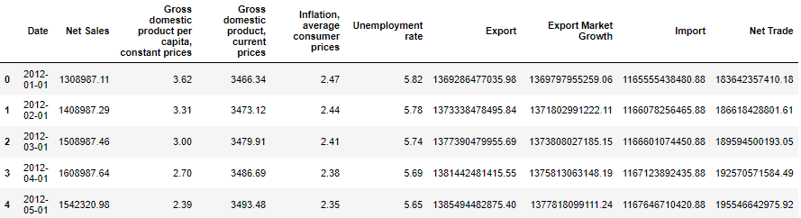
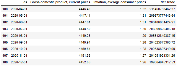
The above table shows several macroeconomic indicators, among which GDP, inflation and unemployment are derived from IMF; Trade data comes from OECD.

3. VAR model predicts net sales in Germany

We will use OECD and IMF as additional factors to predict net monthly sales. Through Granger causality test and Johansen cointegration test, GDP, average consumer price and net trade are filtered out from the eight macroeconomic and trade indicators, which have a linear relationship with monthly sales.

3.1 select the columns selected by Granger causality test and Johansen cointegration test

Cointegration test can be found in another article of the author Timing analysis 15 cointegration sequence
Granger causality test will be briefly introduced later, which may be specially introduced in the next article in the future.

choose_cols = ['Date',
               'Net Sales',
#             'Gross domestic product per capita, constant prices',
            'Gross domestic product, current prices',
            'Inflation, average consumer prices',
#             'Unemployment rate', 
#             'Export',
#             'Export Market Growth', 
#             'Import', 
            'Net Trade'
              ]

masterdf = masterdf[choose_cols]

# ## Keep the masterdf intact, select current data until March as current data

alldf = masterdf.copy()
alldf.index = pd.DatetimeIndex(alldf.Date)
alldf = alldf.sort_index()

### fill any missing values on previous date using backfill
alldf = alldf.fillna(method='bfill')

alldf.index = pd.DatetimeIndex(alldf.Date)
alldf = alldf[alldf.index < '2020-04-01']
alldf = alldf.reset_index(drop=True)

## we rename date as 'ds' and Net Sales as 'y'
## Prophet makes it compulsory to rename these columns as such
alldf = alldf.rename(columns={'Date':'ds',
                     'Net Sales':'y'
                     })
# alldf['ds'] = pd.to_datetime(alldf['ds'])

tsdf = alldf.copy()
tsdf['ds'] = pd.to_datetime(tsdf['ds'])
tsdf.index = pd.DatetimeIndex(tsdf.ds)
tsdf = tsdf.drop('ds', 1)

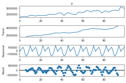
Seasonal decomposition

from statsmodels.tsa.seasonal import seasonal_decompose

result = seasonal_decompose(alldf['y'], model='additive', period=12)
result.plot()

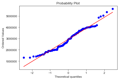
Normal distribution test
Draw QQ plot

from scipy import stats

stat, p = stats.normaltest(tsdf.y)
print('Statistics=%.3f, p=%.3f' % (stat, p))
alpha = 0.05
if p > alpha:
    print('Data looks Gaussian (fail to reject H0)')
else:
    print('Data does not look Gaussian (reject H0)')
    
print('Kurtosis of Normal Dist: {}'.format(stats.kurtosis(tsdf.y)))
print('Skewness of Normal Dist: {}'.format(stats.skew(tsdf.y)))    

stats.probplot(tsdf['y'], plot=plt)

Statistics=3.566, p=0.168
Data looks Gaussian (fail to reject H0)
Kurtosis of Normal Dist: -0.46679521297409465
Skewness of Normal Dist: 0.38404204508729184

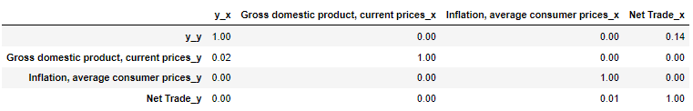
Briefly introduce Granger causality test
Granger causality test is mainly used to test whether one group of practice sequence is the reason affecting another group of practice sequence. Granger causality means that one group of time series data has a significant impact on another group of time series data. The design method is based on regression test. The original assumption is that there is no causality.
The following test method formulates the ssr_chi2test, if this parameter is' params_ftest’, ‘ssr_ftest 'is the F distribution‘ ssr_chi2test 'and' lrtest 'are chi square distributions.

from statsmodels.tsa.stattools import grangercausalitytests
maxlag=12
test = 'ssr_chi2test' 


df = pd.DataFrame(np.zeros((len(tsdf.columns), len(tsdf.columns))), columns=tsdf.columns, index=tsdf.columns)
for c in df.columns:
    for r in df.index:
        test_result = grangercausalitytests(tsdf[[r, c]], maxlag=maxlag, verbose=False)
        p_values = [round(test_result[i+1][0][test][1],4) for i in range(maxlag)]
        min_p_value = np.min(p_values)
        df.loc[r, c] = min_p_value
df.columns = [var + '_x' for var in tsdf.columns]
df.index = [var + '_y' for var in tsdf.columns]

grangerdf = df

grangerdf

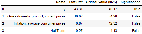
Johanson cointegration test

from statsmodels.tsa.vector_ar.vecm import coint_johansen

alpha = 0.05
out = coint_johansen(tsdf,-1,5)
d = {'0.90':0, '0.95':1, '0.99':2}
traces = out.lr1
cvts = out.cvt[:, d[str(1-alpha)]]
def adjust(val, length= 6): 
    return str(val).ljust(length)

# # Summary
col_name =[]
trace_value = []
cvt_value = []
indicator = []
for col, trace, cvt in zip(tsdf.columns, traces, cvts):
    col_name.append(col)
    trace_value.append(np.round(trace, 2))
    cvt_value.append(cvt)
    indicator.append(trace> cvt)
    
d = {'Name':col_name, 'Test Stat' : trace_value, 'Critical Value (95%)': cvt_value, 'Significance': indicator} 
cj = pd.DataFrame(d)
cj[['Name', 'Test Stat', 'Critical Value (95%)', 'Significance']]

## Split to traning and test
nobs = 10
df_train,df_test = tsdf[0:-nobs],tsdf[-nobs:]
print(df_train.shape)
print(df_test.shape)

(90, 4)
(10, 4)

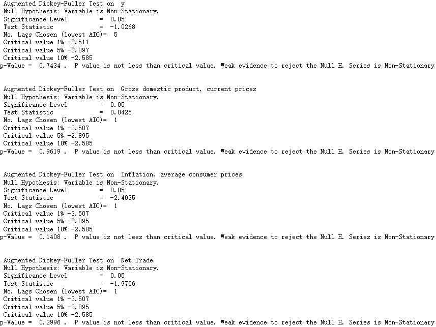
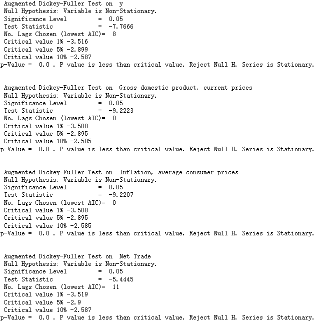
The stability of the training set is tested by the Augmented Dickey Fuller Test

def adf(data,  variable=None, signif=0.05, verbose=False):

    r = adfuller(data, autolag='AIC')
    output = {'test_statistic':np.round(r[0], 4), 'pvalue':np.round(r[1], 4), 'n_lags':np.round(r[2], 4), 'n_obs':r[3]}
    p_value = output['pvalue']

    # Print Summary
    print(' Augmented Dickey-Fuller Test on ', variable)
    print(' Null Hypothesis: Variable is Non-Stationary.')
    print(' Significance Level         = ', signif)
    print(' Test Statistic             = ', output["test_statistic"])
    print(' No. Lags Chosen (lowest AIC)= ', output["n_lags"])

    for key,val in r[4].items():
        print(' Critical value', key, np.round(val, 3))

    if p_value <= signif:
        print("p-Value = ", p_value, ". P value is less than critical value. Reject Null H. Series is Stationary.")
    else:
        print("p-Value = ", p_value, ".  P value is not less than critical value. Weak evidence to reject the Null H. Series is Non-Stationary")

# ADF Test on each column
for name, column in df_train.iteritems():
    adf(column, variable=column.name)
    print('\n')

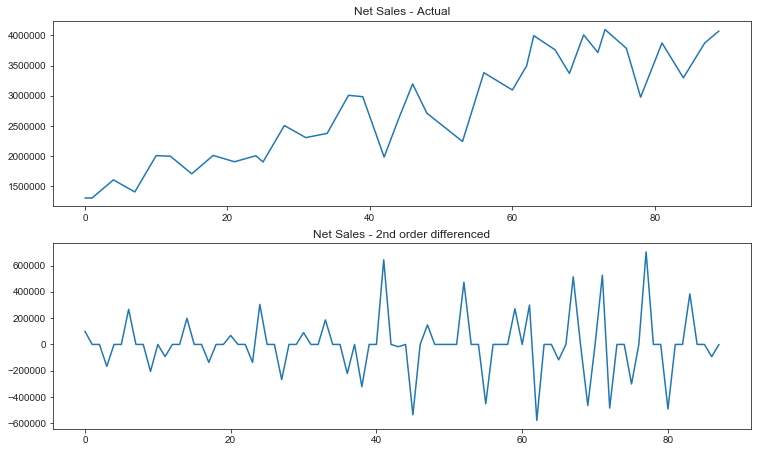
Due to the instability, the first-order and second-order differences are made

# 1st order differencing
df_differenced = df_train.diff().dropna()

# 2nd order differencing
df_differenced = df_differenced.diff().dropna()

fig, ax = plt.subplots(2,1, figsize=(12.5,7.5))

df_train.reset_index()['y'].plot(ax=ax[0])
df_differenced.reset_index()['y'].plot(ax=ax[1])
ax[0].set_title('Net Sales - Actual')
ax[1].set_title('Net Sales - 2nd order differenced')

Text(0.5, 1.0, 'Net Sales - 2nd order differenced')

# ADF Test on each column
for name, column in df_differenced.iteritems():
    adf(column, variable=column.name)
    print('\n')

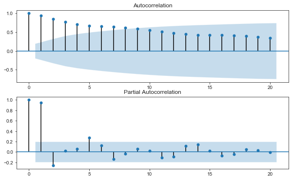
Draw autocorrelation and partial correlation diagrams to further observe the stationarity

from statsmodels.graphics.tsaplots import plot_acf, plot_pacf

fig, ax = plt.subplots(2,1, figsize=(10,6))
plot_acf(tsdf['y'], ax=ax[0])
plot_pacf(tsdf['y'], ax=ax[1])

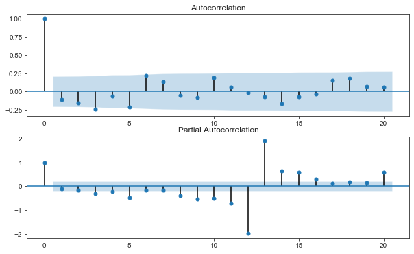
Post difference autocorrelation and partial correlation

from statsmodels.graphics.tsaplots import plot_acf, plot_pacf

fig, ax = plt.subplots(2,1, figsize=(10,6))
plot_acf(df_differenced['y'], ax=ax[0])
plot_pacf(df_differenced['y'], ax=ax[1])

The optimal lag of VAR model is selected by comparing AIC, BIC, FPE and hqic

# call the model and insert the differenced data
model = VAR(df_differenced)
x = model.select_order(maxlags=12)
x.summary()

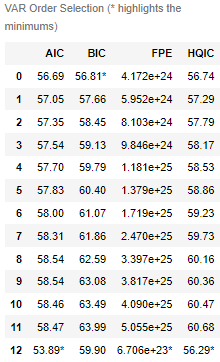
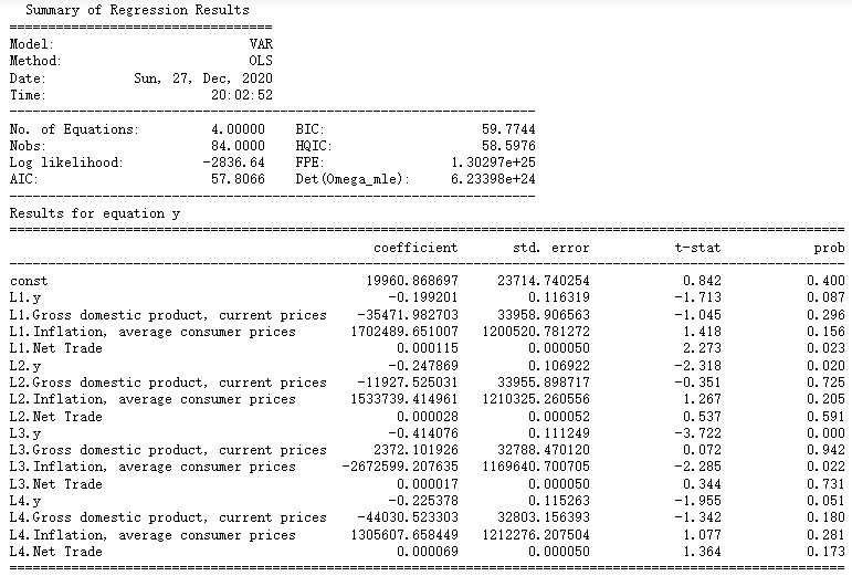
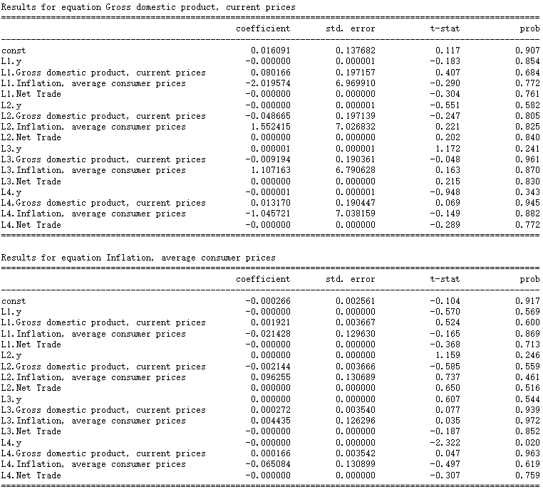
Select lag4

# Select lag4
## lag 4 seems decent, we choose lag 4 and fit it into the model 

model_fitted = model.fit(4)
model_fitted.summary()

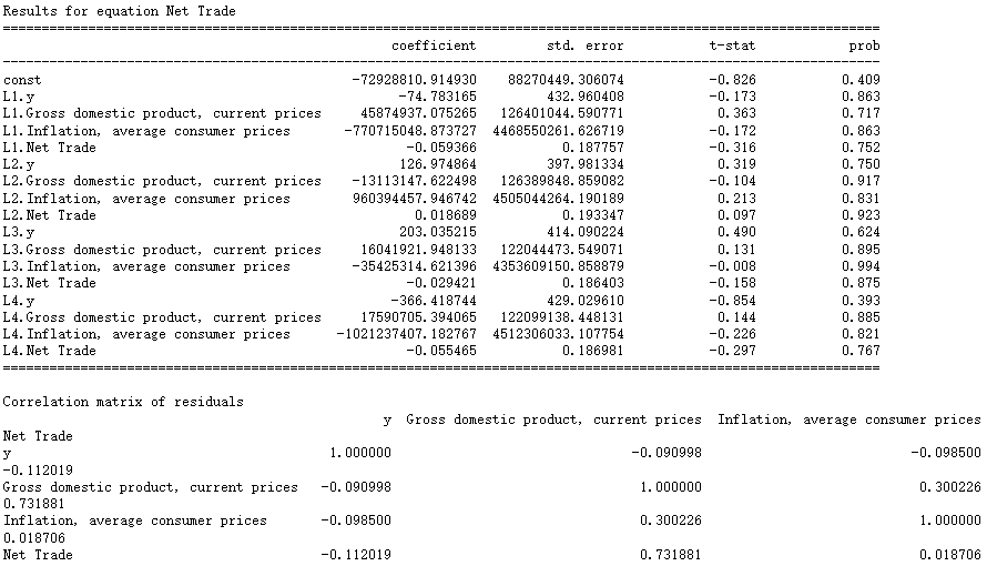
The correlation of residual sequence was tested by Durbin Watson test

from statsmodels.stats.stattools import durbin_watson
out = durbin_watson(model_fitted.resid)

for col, val in zip(tsdf.columns, out):
    print(col, ':', round(val, 2))

y : 2.2
Gross domestic product, current prices : 2.01
Inflation, average consumer prices : 1.98
Net Trade : 2.02

# Get the lag order
lag_order = model_fitted.k_ar
print(lag_order) 

# Separate input data for forecasting
# the goal is to forecast based on the last 4 inputs (since the lag is 4)
forecast_input = df_differenced.values[-lag_order:]

4

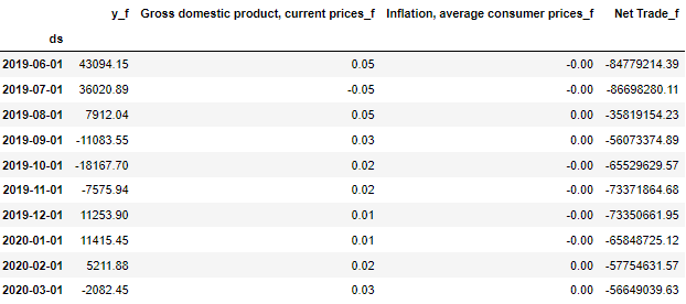
# Forecast
## we insert the last four values and inform the model to predict the next 10 values

fc = model_fitted.forecast(y=forecast_input, steps=nobs)

## organize the output into a clear DataFrame layout, add '_f' suffix at each column indicating they are the forecasted values
df_forecast = pd.DataFrame(fc, index=tsdf.index[-nobs:], columns=tsdf.columns + '_f')
df_forecast

Reverse the data from the difference result to the original data scale

# get a copy of the forecast
df_fc = df_forecast.copy()

# get column name from the original dataframe
columns = df_train.columns

# Roll back from the 1st order differencing
# we take the cumulative sum (from the top row to the bottom) for each of the forecasting data, 
## and the add to the previous step's original value (since we deduct each row from the previous one)
## we rename the new forecasted column with the prefix 'forecast'

# for col in columns: 
#     df_fc[str(col)+'_forecast'] = df_train[col].iloc[-1] + df_fc[str(col)+'_f'].cumsum()

## if you perform second order diff, make sure to get the difference from the last row and second last row of df_train
for col in columns:
    df_fc[str(col)+'_first_differenced'] = (df_train[col].iloc[-1]-df_train[col].iloc[-2]) + df_fc[str(col)+'_f'].cumsum()
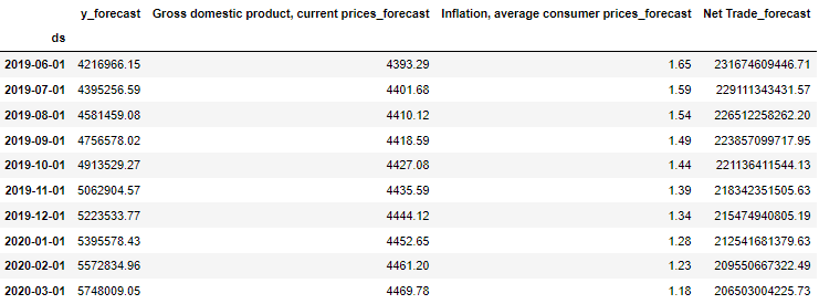
    df_fc[str(col)+'_forecast'] = df_train[col].iloc[-1] + df_fc[str(col)+'_first_differenced'].cumsum()
df_results = df_fc

df_results.loc[:, [ 'y_forecast', 
                    'Gross domestic product, current prices_forecast',     
                    'Inflation, average consumer prices_forecast', 
                    'Net Trade_forecast']]

forecast = df_results['y_forecast'].values
actual = df_test['y']

mae = np.mean(np.abs(forecast - actual))    # MAE
rmse = np.mean((forecast - actual)**2)**.5  # RMSE
mape = np.mean(np.abs(forecast - actual)/np.abs(actual))  # MAPE
print('Mean Absolute Error           : ', mae) 
print('Root Mean Squared Error       : ',rmse)
print('Mean Absolute Percentage Error: ',mape)

Mean Absolute Error : 445641.1508824545
Root Mean Squared Error : 522946.3865355065
Mean Absolute Percentage Error: 0.0999243747966973

## you can use the statsmodels plot_forecast method but the output is not clean
fig = model_fitted.plot_forecast(10)

fig, ax = plt.subplots(figsize=(12, 5))

df_test.reset_index()['y'].plot(color='k', label='Actual')
df_results.reset_index()['y_forecast'].plot(color='r', label='Predicted')

plt.title('VAR Model: Predicted vs Actual on Test Set (June 2019 - Mar 2020)')
ax.legend()

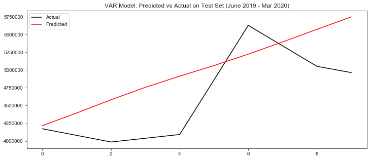
It seems that the prediction result of VAR model is very general.

Apply Prophet

m = Prophet(seasonality_mode='multiplicative',
            growth='linear',
           yearly_seasonality=True,
            mcmc_samples=1000,
            changepoint_prior_scale = 0.001,
            )

Prophet's higher-order function needs to standardize the column name. The time column is named ds and the variable to be predicted is named y.

seasonality_ The mode parameter is set to 'multiplicative', which means that the periodicity is multiplicative, which is compared with 'additive'. Growth = 'linear', which means the growth is linear. Of course, covid-19 can also be designated as logistic growth model, which is also more common, such as economic change cycle, population growth and epidemic model (new crown pneumonia).
weekly_seasonality=False and yearly_seasonality=True. By default, Prophet will use dummy variables to fit weekly_seasonality; Fourier transform is used to fit yearly_seasonality.

mcmc_samples=1000: by default, Prophet will only calculate the uncertainty on the trend, whether the time series is an increasing trend or a decreasing trend. If you want to detect uncertainty periodically, Prophet needs Bayesian sampling. Here, we use 1000 sampling points to estimate the posterior distribution.

changepoint_prior_scale = 0.001: Prophet defines the change point as the abnormal mutation point on the track. If we know that there is a mutation in a certain period, we can customize the mutation point, but by default, prophet will detect it automatically (the default value is 0.05). Here we reduce this value to avoid too many mutation points.

cols = np.array(alldf.columns)
modified_array = np.delete(cols, np.where(cols == 'y'))
modified_array2 = np.delete(modified_array, np.where(modified_array == 'ds'))
alldf_regressor = modified_array2

m.add_regressor('Gross domestic product, current prices', prior_scale=0.5, mode='multiplicative')
m.add_regressor('Inflation, average consumer prices', prior_scale=0.5, mode='multiplicative')
m.add_regressor('Net Trade', prior_scale=0.5, mode='multiplicative')

When we fit the model, we can add other variables detected in the VAR model as additional factors. Because the regression factor must be known in the past and in the future, which means that if we need to predict the data in December, we must know the GDP in the next 12 months, so we used the GDP data predicted by OECD.

m.fit(alldf)

Prepare to forecast the net monthly sales volume from April to December 2020

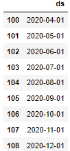
future = m.make_future_dataframe(periods=9, freq='MS')
future.tail(9)

masterdf2 = masterdf.reset_index().rename(columns={'Date':'ds'})
masterdf2['ds'] = pd.to_datetime(masterdf2['ds'])
baseline_future = future.merge(masterdf2.loc[:, modified_array], how='left', on='ds')
baseline_future = baseline_future.fillna(method='ffill')
baseline_future = baseline_future.fillna(method='bfill')
baseline_future.tail(9)

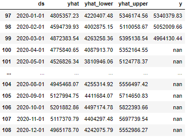
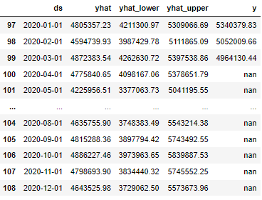
The predicted value is recorded as yhat

forecast = m.predict(baseline_future)

result = pd.concat([forecast[['ds', 'yhat', 'yhat_lower', 'yhat_upper']], alldf[['y']]], 1)
result.tail(12)

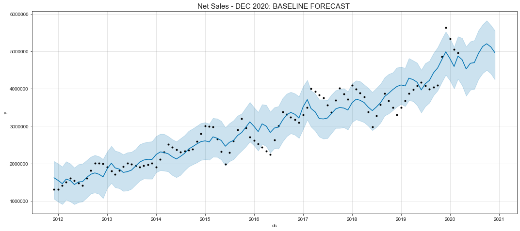
Draw an image
Black dots represent actual data, blue lines represent fitting data, and shaded areas represent uncertainty intervals.

fig, ax = plt.subplots(figsize=(15, 6.5))

m.plot(forecast, ax=ax)
ax.set_title('Net Sales - DEC 2020: BASELINE FORECAST ', size=15)

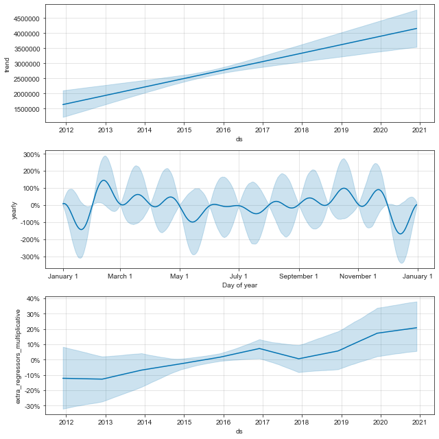
We can observe the main components of the prediction data and get its trend.

m.plot_components(forecast)

Forecast sales growth rate

a = result.loc[pd.DatetimeIndex(result['ds']).year == 2019, 'y'].sum()
b = result.loc[pd.DatetimeIndex(result['ds']).year == 2020, 'yhat'].sum()

(b - a)/ a

0.16700018251482737

Cross validation and performance indicators

from fbprophet.diagnostics import cross_validation
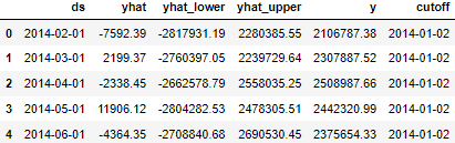
df_cv = cross_validation(m, 
                         initial='730 days', # how many days we want to start training the data
                         period='90 days', # do the forecast every x days (in this case, every quarter)
                         horizon = '270 days'
                        )
df_cv.head()

from fbprophet.diagnostics import performance_metrics
df_p = performance_metrics(df_cv)
df_p.head()

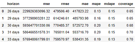
Cross validation of models is very important to evaluate the accuracy of models. By dividing the data into training set and test set, we can estimate the prediction error more accurately. Passing the cross validation data into the performance index function can help us calculate MSE(Mean Squared Error), RMSE(Root Mean Squared Error), MAE(Mean Absolute Error) and MAPE(Mean Absolute Percentage Error) in each period. The first three of the four indicators depend on the scale of the data, while the last one is scale independent.

from fbprophet.plot import plot_cross_validation_metric
plot_cross_validation_metric(df_cv, metric='mape')

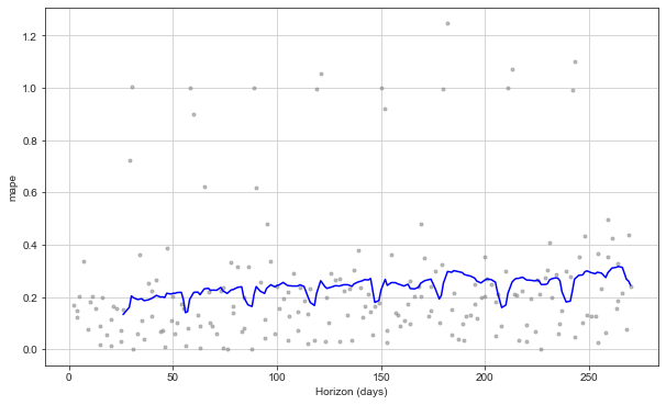
Since MAPE is scale independent, we use this index to judge the model performance. The above figure shows the change of MAPE over time. The minimum is 13%, and the effect is good.

Scene analysis

Now, we want to estimate the impact of the decline in GDP and other economic indicators on sales growth.
Next, we set up a new data frame called future2 to fill in the values of each regression factor, but it will reduce these values by 5%. If we think the economic environment will be worse, we can lower these values a little. Then, the model just trained is used for prediction.

future2 = future.merge(masterdf2.loc[:, modified_array], how='left', on='ds')

future2.iloc[-8:, 1:] = future2.iloc[-8:, 1:].apply(lambda x : x * 0.95)

scenario_forecast = m.predict(future2)
scenario_result = pd.concat([scenario_forecast[['ds', 'yhat', 'yhat_lower', 'yhat_upper']], alldf[['y']]], 1)

future2.iloc[-8:, 1:] = future2.iloc[-8:, 1:].apply(lambda x : x * 0.95)

scenario_forecast = m.predict(future2)
scenario_result = pd.concat([scenario_forecast[['ds', 'yhat', 'yhat_lower', 'yhat_upper']], alldf[['y']]], 1)
scenario_result.tail(12)

fig, ax = plt.subplots(figsize=(15, 6.5))

m.plot(forecast, ax=ax)
ax.set_title('Net Sales - SCENARIO FORECAST UP TO DEC 2020')

a = scenario_result.loc[pd.DatetimeIndex(scenario_result['ds']).year == 2019, 'y'].sum()
b = scenario_result.loc[pd.DatetimeIndex(scenario_result['ds']).year == 2020, 'yhat'].sum()
(b - a) / a

0.11716962913373659

Under this scenario analysis, we predict that the sales growth will be less than 12%.

That's all for this topic. I'll bring more detailed articles about Prophet in the future.