Get more training data (data enhancement)
Data enhancement using geometric transformations
Geometric transformations such as flip, crop, rotation and translation are some commonly used data enhancement techniques.
GAN based data enhancement
Reduce network capacity
The simplest way to prevent overfitting is to reduce the size of the model, that is, the number of learnable parameters in the model (determined by the number of layers and the number of units per layer). In deep learning, the number of learnable parameters in the model is usually called the "capacity" of the model. Intuitively, the model with more parameters has greater "memory ability", so it is easy to learn the perfect dictionary mapping between the training sample and its target, which has no generalization ability. For example, a model with 500000 binary parameters can easily learn the category of each number in MNIST training set: we only need to set 10 binary parameters for each of these 50000 numbers. This model is useless for classifying new digital samples.
Always remember this: deep learning models are often good at fitting training data, but the real challenge is generalization, not fitting.
On the other hand, if the network memory has limited resources, it will not be able to understand this mapping as easily. Therefore, in order to reduce the loss, it will have to resort to learning compression representation. The goal of prediction ability is the type representation we are interested in. At the same time, remember that you should use models with sufficient parameters that are not inappropriate: your model should not lack memory resources. There is a compromise between "too much capacity" and "insufficient capacity".
Unfortunately, there is no magic formula to determine what is the correct number of layers or what is the correct size of each layer. You must evaluate a range of different architectures (in your validation set, not in your test set) to find the right model size for your data. The general process of finding the right model size is to start with relatively few layers and parameters, and then start increasing the size of layers, or adding new layers until you see diminishing returns related to verification losses.
- Our original network is like this:
from keras import models
from keras import layers

original_model = models.Sequential()
original_model.add(layers.Dense(16, activation='relu', input_shape=(10000,)))
original_model.add(layers.Dense(16, activation='relu'))
original_model.add(layers.Dense(1, activation='sigmoid'))

original_model.compile(optimizer='rmsprop',
                       loss='binary_crossentropy',
                       metrics=['acc'])
- Now let's try to replace it with this smaller network:
smaller_model = models.Sequential()
smaller_model.add(layers.Dense(4, activation='relu', input_shape=(10000,)))
smaller_model.add(layers.Dense(4, activation='relu'))
smaller_model.add(layers.Dense(1, activation='sigmoid'))

smaller_model.compile(optimizer='rmsprop',
                      loss='binary_crossentropy',
                      metrics=['acc'])
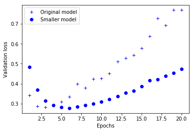
- The following is a comparison of the verification losses of the original network and the smaller network. The point is the verification loss value of the smaller network, and the cross is the initial network (remember: lower verification loss means better model).
original_hist = original_model.fit(x_train, y_train,
                                   epochs=20,
                                   batch_size=512,
                                   validation_data=(x_test, y_test))
maller_model_hist = smaller_model.fit(x_train, y_train,
                                       epochs=20,
                                       batch_size=512,
                                       validation_data=(x_test, y_test))
epochs = range(1, 21)
original_val_loss = original_hist.history['val_loss']
smaller_model_val_loss = smaller_model_hist.history['val_loss']
import matplotlib.pyplot as plt

# b+ is for "blue cross"
plt.plot(epochs, original_val_loss, 'b+', label='Original model')
# "bo" is for "blue dot"
plt.plot(epochs, smaller_model_val_loss, 'bo', label='Smaller model')
plt.xlabel('Epochs')
plt.ylabel('Validation loss')
plt.legend()

plt.show()
#The smaller network starts over fitting than the reference network (after 6 cycles instead of 4 cycles),
#And once the over fitting starts, its performance will decline much slower
Increase normalization
Regularization
In machine learning, we can almost see that an additional item will be added after the loss function. There are generally two kinds of additional items, which are called L1 regularization and L2 regularization in Chinese, or L1 norm and L2 norm.
Description of L1 regularization and L2 regularization:
- L1 regularization refers to the sum of the absolute values of each element in the weight vector w, which is usually expressed as | W||_ one
- L2 regularization refers to the sum of squares of each element in the weight vector w, and then find the square root (it can be seen that the L2 regularization term of Ridge regression has a square sign), which is usually expressed as | W||_ two
Functions of L1 regularization and L2 regularization:
- L1 regularization can generate a sparse weight matrix, that is, a sparse model, which can be used for feature selection
- L2 regularization can prevent model overfitting; To some extent, L1 can also prevent over fitting
from keras import regularizers

# L1 regularization
regularizers.l1(0.001)

# L1 and L2 regularization at the same time
regularizers.l1_l2(l1=0.001, l2=0.001)
--------
Original link: https://blog.csdn.net/jinping_shi/article/details/52433975
Add drop
dropout means that in the training process of deep learning network, the neural network unit is temporarily discarded from the network according to a certain probability. Note that for the time being, for random gradient descent, because it is discarded randomly, each mini batch is training different networks.
Dropout is one of the most effective and commonly used regularization techniques for neural networks, developed by Hinton and his students at the University of Toronto. Dropout, applied to a layer, includes randomly "dropout" (i.e. set to zero) some output features of the layer during training. Suppose that a given layer usually returns a vector [0.2,0.5,1.3,0.8,1.1] for a given input sample during training; After applying dropout, this vector will have several randomly distributed zero terms, such as [0,0.5,1.3,0,1.1]. The "exit rate" is the score of the feature that is zeroed
Usually set between 0.2 and 0.5
During the test, no units are deleted. On the contrary, the output value of this layer is reduced by a factor equal to the deletion rate in order to balance the fact that more units are active than during training.
model.add(layers.Dropout(0.5))
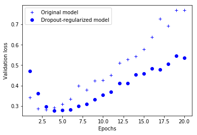
Let's add two Dropout layers to the IMDB network to see how well they do in reducing over fitting
dpt_model = models.Sequential()
dpt_model.add(layers.Dense(16, activation='relu', input_shape=(10000,)))
dpt_model.add(layers.Dropout(0.5))
dpt_model.add(layers.Dense(16, activation='relu'))
dpt_model.add(layers.Dropout(0.5))
dpt_model.add(layers.Dense(1, activation='sigmoid'))

dpt_model.compile(optimizer='rmsprop',
                  loss='binary_crossentropy',
                  metrics=['acc'])
dpt_model_hist = dpt_model.fit(x_train, y_train,
                               epochs=20,
                               batch_size=512,
                               validation_data=(x_test, y_test))
--------
Original link: https://blog.csdn.net/stdcoutzyx/article/details/49022443