1. PCA theory
Common ideas to solve the problem of over fitting: add training to process data, add regularization items, and reduce the dimension of features.
Dimensionality reduction methods: direct feature selection, linear dimensionality reduction (PCA, MDS) and nonlinear dimensionality reduction (manifold).
1.1 representation of mean and variance of high-dimensional samples
Given the Data matrix,
X
=
(
x
1
,
x
2
,
.
.
.
,
x
N
)
N
∗
p
T
X=(x_1,x_2,...,x_N)^{T}_{N*p}
X=(x1,x2,...,xN)N∗pT.
Mean value of sample characteristics:
X
‾
p
∗
1
=
1
N
∑
i
=
1
N
x
i
\overline{X}_{p*1}= \frac{1}{N}\sum_{i=1}^Nx_i
Xp∗1=N1i=1∑Nxi
Sample characteristic variance:
S
p
∗
p
=
1
N
∑
i
=
1
N
(
x
i
−
X
‾
)
(
x
i
−
X
‾
)
T
S_{p*p}=\frac{1}{N}\sum_{i=1}^N(x_i-\overline{X})(x_i-\overline{X})^{T}
Sp∗p=N1i=1∑N(xi−X)(xi−X)T
Then there is the representation of the mean and variance of high-dimensional samples:
X
‾
p
∗
1
=
1
N
∑
i
=
1
N
x
i
\overline{X}_{p*1}= \frac{1}{N}\sum_{i=1}^Nx_i
Xp∗1=N1∑i=1Nxi
=
1
N
(
x
1
,
x
2
,
.
.
.
,
x
N
)
(
1
.
.
.
1
)
N
∗
1
= \frac{1}{N}(x_1,x_2,...,x_N)\begin{pmatrix} 1 \\ ...\\ 1 \\ \end{pmatrix}_{N*1}
=N1(x1,x2,...,xN)⎝⎛1...1⎠⎞N∗1
=
1
N
X
T
1
N
∗
1
= \frac{1}{N}X^{T}1_{N*1}
=N1XT1N∗1
S
p
∗
p
=
1
N
∑
i
=
1
N
(
x
i
−
X
‾
)
(
x
i
−
X
‾
)
T
S_{p*p}=\frac{1}{N}\sum_{i=1}^N(x_i-\overline{X})(x_i-\overline{X})^{T}
Sp∗p=N1∑i=1N(xi−X)(xi−X)T
=
1
N
(
x
1
−
X
‾
,
.
.
.
,
x
N
−
X
‾
)
(
(
x
1
−
X
‾
)
T
.
.
.
(
x
N
−
X
‾
)
T
)
N
∗
1
=\frac{1}{N}(x_1-\overline{X},...,x_N-\overline{X})\begin{pmatrix} (x_1-\overline{X})^{T} \\ ...\\ (x_N-\overline{X})^{T}\\ \end{pmatrix}_{N*1}
=N1(x1−X,...,xN−X)⎝⎛(x1−X)T...(xN−X)T⎠⎞N∗1
=
1
N
X
T
(
I
N
−
1
N
1
N
1
N
T
)
N
X
T
(
I
N
−
1
N
1
N
1
N
T
)
T
X
=\frac{1}{N}X^T(I_N-\frac{1}{N}1_N1_N^T){N}X^T(I_N-\frac{1}{N}1_N1_N^T)^TX
=N1XT(IN−N11N1NT)NXT(IN−N11N1NT)TX
If the expression in parentheses is regarded as H, there are:
=
1
N
X
T
H
H
T
X
=\frac{1}{N}X^THH^TX
=N1XTHHTX
You can try to calculate and find:
H
T
=
H
H^T=H
HT=H
H
n
=
H
H^n=H
Hn=H
Then there are:
S
p
∗
p
=
1
N
X
T
H
X
S_{p*p}=\frac{1}{N}X^THX
Sp∗p=N1XTHX
1.2 maximum projection variance & minimum reconstruction distance
classical PCA can be regarded as:
One center: reconstruction of original feature space
→
\to
→ irrelevant);
Two basic points: 1 Maximum projection variance 2 Minimum reconstruction distance
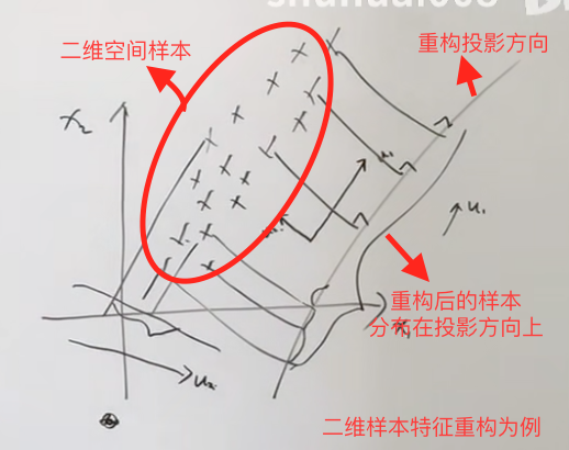
The basic idea is to project the original features in one direction. The idea is a bit like but different from LDA linear discriminant analysis. If there are relevant problems that need to be reviewed, LDA will write another LDA note. It maximizes the variance of the new samples obtained in the projection direction of the sample features, and enables the new sample data to be distinguished, and the possibility of reconstruction is as large as possible. As shown in the figure:

Centralization:
x
i
−
X
‾
x_i-\overline{X}
xi−X
The projection direction is:
u
1
⃗
\vec{u_1}
u1
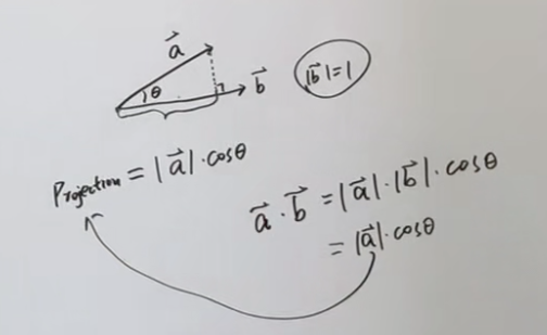
According to the projection theorem shown in the figure, there are:
J
=
(
∑
i
=
1
N
(
x
i
−
X
‾
)
T
u
1
⃗
)
2
J=(\sum_{i=1}^N(x_i-\overline{X})^T\vec{u_1})^2
J=(∑i=1N(xi−X)Tu1
)2
=
J
=
∑
i
=
1
N
u
1
⃗
T
(
x
i
−
X
‾
)
(
x
i
−
X
‾
)
T
u
1
⃗
=J=\sum_{i=1}^N\vec{u_1}^T(x_i-\overline{X})(x_i-\overline{X})^T\vec{u_1}
=J=∑i=1Nu1
T(xi−X)(xi−X)Tu1
=
u
1
⃗
T
(
∑
i
=
1
N
1
N
(
x
i
−
X
‾
)
(
x
i
−
X
‾
)
T
)
u
1
⃗
=\vec{u_1}^T(\sum_{i=1}^N\frac{1}{N}(x_i-\overline{X})(x_i-\overline{X})^T)\vec{u_1}
=u1
T(∑i=1NN1(xi−X)(xi−X)T)u1
=
u
1
⃗
T
S
u
1
⃗
=\vec{u_1}^TS\vec{u_1}
=u1
TSu1

Then the solution of PCA can be regarded as an optimization problem with constraints:
{
u
1
′
=
a
r
g
m
a
x
u
1
T
S
u
1
s
.
t
.
u
1
T
u
1
=
1
\begin{cases} u_1'=argmaxu_1^TSu_1\\ s.t.u_1^Tu_1=1\\ \end{cases}
{u1′=argmaxu1TSu1s.t.u1Tu1=1
According to Lagrange multiplier method:
f
(
u
,
λ
)
=
u
1
T
S
u
1
+
λ
(
u
1
T
u
1
−
1
)
f(u,\lambda)=u_1^TSu_1+\lambda(u_1^Tu_1-1)
f(u,λ)=u1TSu1+λ(u1Tu1−1)
Partial derivation:
∂
f
∂
u
1
=
2
S
u
1
−
λ
2
u
1
=
0
\frac{\partial f}{\partial u_1}=2Su_1-\lambda2u_1=0
∂u1∂f=2Su1−λ2u1=0
Then there are:
S
u
1
=
λ
u
1
Su_1=\lambda u_1
Su1=λu1
It can be seen that PCA is actually the reconstruction of feature space. For each direction selected, there is a corresponding eigenvalue. The new reconstructed coordinate system is
u
1
,
u
2
,
.
.
.
,
u
p
u_1,u_2,...,u_p
u1,u2,..., up, then each centralized reconstructed sample can be expressed as:
x
i
=
∑
k
=
1
p
(
x
i
T
u
k
)
u
k
x_i=\sum_{k=1}^p(x_i^Tu_k)u_k
xi=k=1∑p(xiTuk)uk
Dimensionality reduction is to preserve the spatial dimension according to the needs of the reconstructed feature space samples
p
p
Select from p spaces
q
q
If q dimensions are reserved, the sample after dimension reduction is expressed as:
x
i
′
=
∑
k
=
1
q
(
x
i
T
u
k
)
u
k
x_i'=\sum_{k=1}^q(x_i^Tu_k)u_k
xi′=k=1∑q(xiTuk)uk
Then the minimum reconstruction cost can be expressed as:
J
=
1
N
∑
i
=
1
N
∣
∣
x
i
−
x
i
′
∣
∣
2
=
1
N
∑
k
=
q
+
1
p
∣
∣
x
i
−
x
i
′
∣
∣
2
J=\frac{1}{N}\sum_{i=1}^{N}||x_i-x_i'||^2=\frac{1}{N}\sum_{k=q+1}^{p}||x_i-x_i'||^2
J=N1i=1∑N∣∣xi−xi′∣∣2=N1k=q+1∑p∣∣xi−xi′∣∣2
=
1
N
∑
i
=
1
N
∑
k
=
q
+
1
p
(
x
i
T
u
k
)
2
=\frac{1}{N}\sum_{i=1}^{N}\sum_{k=q+1}^{p}(x_i^Tu_k)^2
=N1i=1∑Nk=q+1∑p(xiTuk)2
Consider centralization:
=
1
N
∑
i
=
1
N
∑
k
=
q
+
1
p
(
(
x
i
−
X
‾
)
T
u
k
)
2
=\frac{1}{N}\sum_{i=1}^{N}\sum_{k=q+1}^{p}((x_i-\overline{X})^Tu_k)^2
=N1i=1∑Nk=q+1∑p((xi−X)Tuk)2
=
∑
k
=
q
+
1
p
∑
i
=
1
N
1
N
(
(
x
i
−
X
‾
)
T
u
k
)
2
=
∑
k
=
q
+
1
p
u
k
T
S
u
k
=\sum_{k=q+1}^{p}\sum_{i=1}^{N}\frac{1}{N}((x_i-\overline{X})^Tu_k)^2=\sum_{k=q+1}^{p}u_k^TSu_k
=k=q+1∑pi=1∑NN1((xi−X)Tuk)2=k=q+1∑pukTSuk
Therefore, PCA will get the same result from two perspectives.
2. PCA practice
The dimensionality reduction algorithms in sklearn are included in the decomposition module.
2.1 important parameters n_components
Represents the dimension required after dimension reduction, that is, the number of features to be retained after dimension reduction.
2.1.1 visual feature distribution of high-dimensional data
Reduce the dimension of the feature to 3D (if necessary).
import matplotlib.pyplot as plt
from sklearn.datasets import load_iris
from sklearn.decomposition import PCA
iris = load_iris()
y = iris.target
X = iris.data
import pandas as pd
print(pd.DataFrame(X))

pca = PCA(n_components=2)
pca = pca.fit(X) # Fitting model
X_dr = pca.transform(X) # Get new matrix
# One step: X_dr = PCA(2).fit_transform(X)

# Take out the first feature of the sample data classified as 0
X_dr[y == 0, 0]
# Take out the second feature of the sample data classified as 0
X_dr[y == 0, 2]

# Draw, or cycle
plt.figure()
plt.scatter(X_dr[y==0, 0], X_dr[y==0, 1], c="red", label=iris.target_names[0])
plt.scatter(X_dr[y==1, 0], X_dr[y==1, 1], c="black", label=iris.target_names[1])
plt.scatter(X_dr[y==2, 0], X_dr[y==2, 1], c="orange", label=iris.target_names[2])
plt.legend()
plt.title("PCA of IRIS dataset")
plt.show()

# View the interpretability variance size of the new feature
print(pca.explained_variance_)
# View the contribution rate of interpretable variance of new features (the proportion of original information carried by each new feature)
print(pca.explained_variance_ratio_)
# View the total proportion of reduced dimension information in the original information
print(pca.explained_variance_ratio_.sum())

import numpy as np
# Accumulate the list
np.consum(pca.explained_variance_ratio_)
2.1.2 select n by other methods_ components
# Maximum likelihood estimation can be used to take n_ Value of components
pca_mle = PCA(n_components="mle")
pca_mle = pca_mle.fit(X)
X_mle = pca_mle.transform(X)

# Select n according to the proportion of information_ components
pca_f = PCA(n_componets=0.97, svd_solver="full")
pca_f = pca_f.fit(X)
X_f = pca_f.transform(X)
2.2 parameter SVD_ solver&random_ state
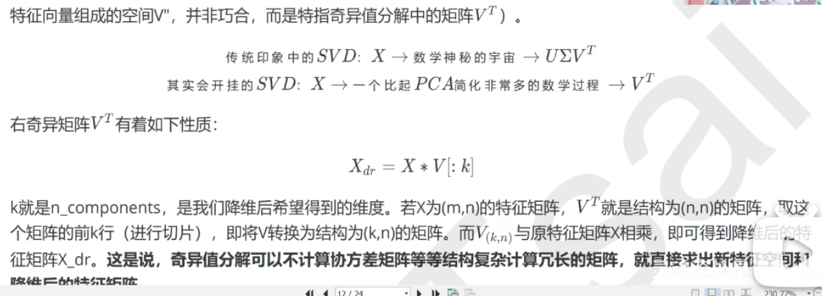
PCA can also be viewed from the perspective of singular value decomposition:

svd_ There are four kinds of solvers: auto (full for small amount of data, and randomized for large amount of data), full (complete decomposition of singular value matrix), arpack (it can accelerate the operation, which is suitable for large and sparse characteristic matrix), and randomized (it is suitable for large characteristic matrix and large amount of calculation).
2.3 important attribute components_
from sklearn.datasets import fetch_lfw_people
from sklearn.decomposition import PCA
import matplotlib.pyplot as plt
import numpy as np
faces = fetch_lfw_people(min_faces_per_people=60)
X = faces.data

# Realistic rendering of images in a dataset
# 4 rows and 5 columns 4 * 5 = 20 drawings
# figsize is the canvas size
fig, axes = plt.subplot(4, 5, figsize=(8, 4), subplot_kw={"xticks":[], "yticks":[]})# Do not display axes
for i, ax in enumerate(axes.flat):
	ax.imshow(faces.images[i,:,:], cmap="gray")

pca = PCA(150).fit(X)
V = pca.components_
# Visual components_ Core information
fig, axes = plt.subplot(3, 8, figsize=(8, 4), subplot_kw={"xticks":[], "yticks":[]})# Do not display axes
for i, ax in enumerate(axes.flat):
	ax.imshow(V[i,:].reshape(62,47), cmap="gray")
2.4 important interface reverse_ transform
Dimensionality reduction is irreversible and cannot be recovered even with this interface.
X_inverse = pca.inverse_transform(X_dr)
fig, axes = plt.subplot(2, 10, figsize=(10, 2.5), subplot_kw={"xticks":[], "yticks":[]})# Do not display axes
for i in range(10):
	ax[0,i].imshow(faces.images[i,:,:], cmap="binary_r")
	ax[1,i].imshow(X_inverse[i].reshape(62,47), cmap="binary_r")
2.5 noise filtering with PCA
from sklearn.datasets import load_digits

digits = load_digits()
# View label
print(set(digits.target.tolist()))
# mapping
def plot(data):
	fig, axes = plt.subplot(4, 10, figsize=(10, 4), subplot_kw={"xticks":[], "yticks":[]})# Do not display axes
	for i, ax in enumerate(axes.flat):
		ax.imshow(data[i].reshape(8,8), cmap="binary")

# Add noise to the data
np.random.RandomState(42)
noisy = np.random.normal(digits.data, 2)
plot(noisy)

pca = PCA(0.5, svd_solver="full").fit(noisy)
X_dr = pca.transform(noisy)

witout_noise = pca.inverse_transform(X_dr)
plot(without_noise)
2.6 actual combat: dimension reduction of handwritten data set
The packages that have been imported will not be imported.
from sklearn.esemble import RandomForestClassifier as RFC
from sklearn.model_selection import cross_val_score
data = pd.read_csv("data set CSV route")
X = data.iloc[:, 1:]
y = data.iloc[:,0]

# Draw the cumulative variance contribution rate curve to find the best dimension range after dimension reduction
pca_line = PCA().fit(X)
plt.figure(figsize=[20,5])
plt.plot(np.consum(pca.line.explained_variance_ratio_))
plt.xlabel("number of components after dimension reduction")
plt.ylabel("cumulative explained variance")
plt.show()

# The learning curve after dimension reduction continues to narrow the range of the best dimension
score = []
# Reduce the range (10, 25) and draw the learning curve again
for i in range(1, 101, 10):
	X_dr = PCA(i).fit_transform(X)
	once = cross_val_score(RFC(n_estimator=10, random_state=0), X_dr, y, cv=5).mean()
	score.append(once)
plt.figure(figsize=[20,5])
plt.plot(range(1, 101, 10), score)
plt.show()

# Determine the dimension after finding the best parameter
X_dr = PCA(23).fit_transform(X)
cross_val_score(RFC(n_estimator=100, random_state=0), X_dr, y, cv=5).mean()

# Use KNN to train
from sklearn.neighbors import KNeighborsClassifier as KNN
cross_val_score(KNN(), X_dr, y, cv=5).mean()

# k-value learning curve of KNN
score = []
# Determine the value of k as 3
for i in range(10):
	X_dr = PCA(23).fit_transform(X)
	once = cross_val_score(KNN(i+1), X_dr, y, cv=5).mean()
	score.append(once)
plt.figure(figsize=[20,5])
plt.plot(range(10), score)
plt.show()