Project training (XI)
This paper records the use of logistic regression in the project
logistic regression
Logistic regression is one of many classification algorithms. Usually, logistic regression is used for binary problems, such as predicting whether it will rain tomorrow. Of course, it can also be used for multi classification problems.
Assuming that there are some data points, we use a straight line to fit these points (the line is called the best fitting straight line), and this fitting process is called regression, as shown in the figure below: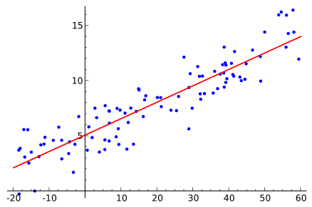
Logistic regression is a classification method, which uses the characteristic that the threshold of Sigmoid function is [0,1]. The main idea of logistic regression classification is to establish a regression formula for the classification boundary line according to the existing data. In fact, logistic is essentially a discriminant model based on conditional probability.
So to understand Logistic regression, we must first look at the Sigmoid function, which we can also call Logistic function.
The following picture shows us what the Sigmoid function looks like.
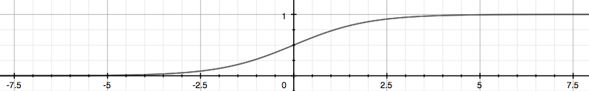
Z is a matrix, θ Is the parameter column vector (required solution), and X is the sample column vector (given data set). θ^ T represents θ Transpose of. g(z) function realizes the mapping of any real number to [0,1], so that our data set ([x0,x1,..., xn]) can be mapped to [0,1] interval for classification whether it is greater than 1 or less than 0. h θ (x) The probability that the output is 1 is given. For example, when H θ (x)=0.7, then there is a 70% probability that the output is 1. The probability of output 0 is the complement of output 1, that is, 30%.
If we have the appropriate parameter column vector θ ([ θ 0 θ 1,… θ n]^T), and the sample column vector x([x0,x1,..., xn]), then we can calculate a probability through the above formula for the classification of sample X. if the probability is greater than 0.5, we can say that the sample is a positive sample, otherwise the sample is a negative sample.
For example, for the "spam discrimination problem", for a given email (sample), we define non spam as positive and spam as negative. We can determine whether the email is spam by calculating the probability value.
So here comes the question...! How to get the appropriate parameter vector θ?
According to the characteristics of sigmoid function, we can make the following assumptions:

The formula is in the known sample X and parameters θ In this case, the sample x attribute is the conditional probability of positive samples (y=1) and negative samples (y=0). Ideally, according to the above formula, the probability of each point is 1, that is, the complete classification is correct. However, considering the actual situation, the closer the probability of sample points is to 1, the better the classification effect is. For example, if the probability of a sample belonging to a positive sample is 0.51, we can explain that the sample belongs to a positive sample. The probability that another sample belongs to the positive sample is 0.99, so we can also explain that this sample belongs to the positive sample. But obviously, the second sample has a higher probability and is more persuasive. We can combine the above two probability formulas into one:

The combined Loss function is called Loss function. When y is equal to 1, item (1-y) (second item) is 0; When y equals 0, the Y term (the first term) is 0. To s simplify the problem, we calculate the logarithm of the whole expression (logarithm of exponential problem is a common method to deal with mathematical problems):

This loss function is for a sample. Given a sample, we can calculate the probability of the category to which the sample belongs through this loss function, and the greater the probability, the better. Therefore, we can solve the maximum value of this loss function. Now that the probability comes out, it's time for the maximum likelihood estimation to come out. Assuming that samples and samples are independent of each other, the probability of generating the whole sample set is the product of the probability of generating all samples, and the following formula can be obtained:
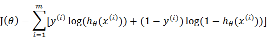
Where, m is the total number of samples, y(i) represents the category of the ith sample, and x(i) represents the ith sample. It should be noted that θ Is a multidimensional vector, and x(i) is also a multidimensional vector.
To sum up, J( θ) The largest θ Value is the model we need to solve.
How to solve J( θ) maximal θ What's the value? Because it is to find the maximum value, we need to use the gradient rise algorithm. If the problem is to solve J( θ) least θ Value, then we need to use the gradient descent algorithm. In the face of our problem, if J( θ) := - J( θ), Then the problem is transformed from maximum to minimum, and the algorithm used is changed from gradient rising algorithm to gradient falling algorithm. Their ideas are the same. If you learn one, you will learn the other. In this paper, the gradient rise algorithm is used to solve it.
Gradient rise
Do it in an iterative way. It's like climbing a slope, approaching the extreme value bit by bit. This method of finding the best fitting parameters is the optimization algorithm. The action of climbing a slope is expressed by a mathematical formula, which is:
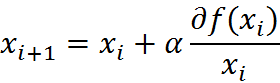
Among them, α For the step size, that is, the learning rate, control the amplitude of the update.
General process
Data collection: use any method to collect data.
Prepare data: since distance calculation is required, the data type is required to be numerical. In addition, the structured data format is the best.
Analyze data: use any method to analyze the data.
Training algorithm: most of the time will be used for training. The purpose of training is to find the best classification regression coefficient.
Test algorithm: once the training steps are completed, the classification will be fast.
Using algorithm: first, we need to input some data and convert it into corresponding structured values; Then, based on the trained regression coefficients, these values can be simply regressed to determine which category they belong to; After that, we can do some other analysis work on the output categories.
application
In the project, the sklearn library is used to directly use the functions inside to realize the logical regression classifier
from sklearn.linear_model import LogisticRegression
import numpy as np
import random

# Logistic regression is a binary classification algorithm, which uses the characteristic that the threshold of Sigmoid function is [0,1].
# The main idea of Logistic regression classification is to establish a regression formula for the classification boundary line according to the existing data.
# Find parameter vector θ, Realize SIGMOD classification
def sigmoid(inX):
    return 1.0 / (1 + np.exp(-inX))

def stocGradAscent1(dataMatrix, classLabels, numIter=150):
    m, n = np.shape(dataMatrix)  # Returns the size of the dataMatrix. m is the number of rows and n is the number of columns.
    weights = np.ones(n)  # Parameter initialization										#Store regression coefficients for each update
    for j in range(numIter):
        dataIndex = list(range(m))
        for i in range(m):
            alpha = 4 / (1.0 + j + i) + 0.01  # Reduce the size of alpha by 1/(j+i) each time.
            randIndex = int(random.uniform(0, len(dataIndex)))  # Randomly selected samples
            h = sigmoid(sum(dataMatrix[randIndex] * weights))  # Select a randomly selected sample and calculate h
            error = classLabels[randIndex] - h  # calculation error
            weights = weights + alpha * error * dataMatrix[randIndex]  # Update regression coefficient
            del (dataIndex[randIndex])  # Delete used samples
    return weights  # return


def gradAscent(dataMatIn, classLabels):
    dataMatrix = np.mat(dataMatIn)  # mat converted to numpy
    labelMat = np.mat(classLabels).transpose()  # Convert to numpy mat and transpose it
    m, n = np.shape(dataMatrix)  # Returns the size of the dataMatrix. The number of rows n is m.
    alpha = 0.01  # The moving step size, that is, the learning rate, controls the amplitude of the update.
    maxCycles = 500  # Maximum number of iterations
    weights = np.ones((n, 1))
    for k in range(maxCycles):
        h = sigmoid(dataMatrix * weights)  # Gradient rise vectorization formula
        error = labelMat - h
        weights = weights + alpha * dataMatrix.transpose() * error
    return weights.getA()  # Converts a matrix to an array and returns

def colicTest():
    frTrain = open('horseColicTraining.txt')  # Open training set
    frTest = open('horseColicTest.txt')  # Open test set
    trainingSet = [];
    trainingLabels = []
    for line in frTrain.readlines():
        currLine = line.strip().split('\t')
        lineArr = []
        for i in range(len(currLine) - 1):
            lineArr.append(float(currLine[i]))
        trainingSet.append(lineArr)
        trainingLabels.append(float(currLine[-1]))
    trainWeights = stocGradAscent1(np.array(trainingSet), trainingLabels, 500)  # Using improved random ascending gradient training
    errorCount = 0;
    numTestVec = 0.0
    for line in frTest.readlines():
        numTestVec += 1.0
        currLine = line.strip().split('\t')
        lineArr = []
        for i in range(len(currLine) - 1):
            lineArr.append(float(currLine[i]))
        if int(classifyVector(np.array(lineArr), trainWeights)) != int(currLine[-1]):
            errorCount += 1
    errorRate = (float(errorCount) / numTestVec) * 100  # Error rate calculation
    print("The test set error rate is: %.2f%%" % errorRate)


def classifyVector(inX, weights):
    prob = sigmoid(sum(inX * weights))
    if prob > 0.5:
        return 1.0
    else:
        return 0.0

def loadDataSet(vecfileName, labelfileName, num1, num2):
    dataMat = [];
    labelMat = []
    fr = open(vecfileName)
    for line in fr.readlines()[num1:num2]:
        tmp_vec = eval(line[5:-2])
        dataMat.append(tmp_vec)
    fr = open(labelfileName)
    for line in fr.readlines()[num1:num2]:
        tmp_label = int(line[2])
        labelMat.append(tmp_label)

    return dataMat, labelMat

def loadDataSet2(fileName ,num1, num2):
    dataMat = [];
    labelMat = []
    fr = open(fileName)
    for line in fr.readlines()[num1:num2]:
        print(line)
    return dataMat, labelMat

def colicSklearn():
    trainingSet ,trainingLabels = loadDataSet("vec_clean.csv","label_clean.csv",0,9000)
    testSet ,testLabels = loadDataSet("vec_clean.csv","label_clean.csv",9001,9999)
    classifier = LogisticRegression(solver='sag', max_iter=800,multi_class='multinomial').fit(trainingSet, trainingLabels)
    test_accurcy = classifier.score(testSet, testLabels) * 100
    print('Correct rate:%f%%' % test_accurcy)

if __name__ == '__main__':
    colicSklearn()
After adjusting parameters, the accuracy of text three classification in the project can reach more than 70%
reference resources
https://cuijiahua.com/blog/2017/11/ml_6_logistic_1.html
https://cuijiahua.com/blog/2017/11/ml_7_logistic_2.html