Prometheus monitoring system
Introduction to Prometheus
Prometheus is an open source system monitoring and alarm toolkit, originally built on SoundCloud. Since its establishment in 2012, many companies and organizations have adopted Prometheus, which has a very active developer and user community. It is now an independent open source project, independent of any company for maintenance. In order to emphasize this point and clarify the governance structure of the project, Prometheus joined the cloud native Computing Foundation in 2016 as the second hosting project after Kubernetes.
Prometheus collects and stores its indicators as time series data, that is, the indicator information is stored together with the timestamp recording it, and an optional key value pair called a tag.
Prometheus features
- Multidimensional data model composed of indicator name and time series identified by key value pair label.
- PromQL, a powerful query language.
- Independent of distributed storage, a single service node has autonomy.
- The time series data is actively pulled by the server through HTTP protocol.
- Intermediate gateway is used to push time series data.
- Discover targets through service discovery or static configuration files.
- Multiple types of icons and dashboards are supported.
Prometheus component
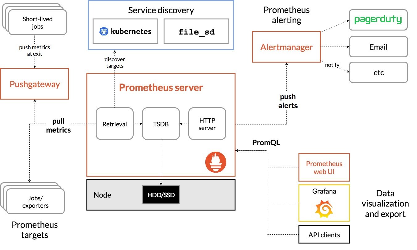
Prometheus Server is responsible for the collection and storage of time series index data, but Prometheus Server is not responsible for data analysis, aggregation, visual display and alarm.
Prometheus ecosystem contains many components, some of which are optional:
- Prometheus Server: collect and store time series data;
- Client Library: client library, which provides a development path for applications that expect to provide native Instrumentation functions;
- Push Gateway: a gateway that receives indicator data usually generated by short-term jobs and supports indicator pulling by Prometheus Server;
- Exporters: indicators used to expose existing applications or services (Instrumentation is not supported) to Prometheus Server;
- Alertmanager: after receiving the alarm notification from Prometheus Server, it sends the alarm information to the user efficiently through preprocessing functions such as de duplication, grouping and routing;
- Data Visualization: Prometheus Web UI (built in Prometheus Server), Grafana, etc;
- Service Discovery: dynamically discover the Target to be monitored, which is an important component to complete the monitoring configuration, especially in a container environment (Prometheus Server built-in).
The overall architecture and ecological components of Prometheus are shown in the figure below:
Prometheus data model
All monitoring data collected by Prometheus are stored in the built-in time series database (TSDB) in the form of indicators (Metric), belonging to the same indicator name, the same label set and time stamped data stream. In addition to the stored time series, Prometheus can also generate temporary and derived time series as the return result according to the query request.
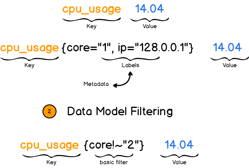
Indicator name and label
Each time series is uniquely identified by the indicator name and a set of labels (key value pairs). The indicator name can reflect the meaning of the monitored sample (for example, cpu_usage{core="1", ip=""128.0.0.1} 14.04 indicates the use of the current system core 1). The indicator name can only be composed of ASCII characters, numbers, underscores and colons, and must match the positive expression [a-za-z:] [a-za-z0-9:] *.
[note] colons are used to identify user-defined record rules. Colons cannot be used in exporter s or indicators directly exposed by monitoring objects to define indicator names.
Prometheus opens a powerful multidimensional data model by using tags: for the same indicator name, specific measurement dimension instances will be formed through the collection of different tag lists (for example, all http requests with the measurement name of / api/tracks and labeled with method=POST will form specific http requests). The query language filters and aggregates these indicators and tag lists. Changing any tag value on any metric (including adding or deleting metrics) will create a new time series.
The label name can only be composed of ASCII characters, numbers and underscores, and satisfies the regular expression [a-za-z] [a-za-z0-9] *. Among them__ Tags as prefixes are keywords exposed by the system and can only be used within the system. The value of the tag can contain any Unicode encoded character.
sample
Each point in the time system is called a sample. The sample consists of the following three parts:
- metric: indicator name and labelsets describing the characteristics of the current sample;
- Timestamp: a timestamp accurate to milliseconds;
- Sample value: a folat64 floating-point data represents the value of the current sample.
Representation of sample value:
<metric name>{<label name>=<label value>, ...}
Indicator type of Prometheus
Prometheus provides four core indicator types in its client library. However, these types are only in the client library (the client can call different API interfaces according to different data types) and online protocols. In fact, the Prometheus server does not distinguish the indicator types, but simply regards these indicators as untyped time series.
Prometheus Go client documentation
Counter
Counter is an indicator of monotonically increasing sample data (only increasing but not decreasing, and cannot be negative), which can be used to represent the number of interface calls, site visits, error occurrences, etc.
Gauge (instrument cluster)
Gauge is used to store index data with fluctuation characteristics (which can be increased or decreased), such as memory space utilization, concurrent requests, etc.
Histogram (histogram)
In most cases, people tend to use the average value of some quantitative indicators, such as the average utilization of CPU and the average response time of pages. The problem with this method is obvious. Take the average response time of system API calls as an example: if most API requests are maintained within the response time range of 100ms, and the response time of individual requests requires 5s, the response time of some WEB pages will fall to the median, and this phenomenon is called the long tail problem.
In order to distinguish between average slow and long tail slow, the simplest way is to group according to the range of request delay. For example, count the number of requests delayed between 0 and 10ms and the number of requests delayed between 10 and 20ms. In this way, we can quickly analyze the reasons for the slow speed of the system. Histogram and Summary are designed to solve such problems. Through histogram and Summary monitoring indicators, we can quickly understand the distribution of monitoring samples.
Histogram samples the data within a period of time and counts it into the configurable storage bucket. Subsequently, samples can be filtered through the specified interval or the total number of samples can be counted. Finally, the data is generally displayed as a histogram.
Histogram samples provide three indicators (assuming the indicator name is < basename >):
-
The number of sample values distributed in the bucket, named < basename >_ Bucket {Le = "< upper boundary >"}. The explanation is easier to understand. This value indicates that the index value is less than or equal to the number of all samples on the upper boundary.
// Of a total of 2 requests. The number of requests with http request response time < = 0.005 seconds is 0 io_namespace_http_requests_latency_seconds_histogram_bucket{path="/",method="GET",code="200",le="0.005",} 0.0 // Of a total of 2 requests. The number of requests with http request response time < = 0.01 seconds is 0 io_namespace_http_requests_latency_seconds_histogram_bucket{path="/",method="GET",code="200",le="0.01",} 0.0 // Of a total of 2 requests. The number of requests with http request response time < = 0.025 seconds is 0 io_namespace_http_requests_latency_seconds_histogram_bucket{path="/",method="GET",code="200",le="0.025",} 0.0 io_namespace_http_requests_latency_seconds_histogram_bucket{path="/",method="GET",code="200",le="0.05",} 0.0 io_namespace_http_requests_latency_seconds_histogram_bucket{path="/",method="GET",code="200",le="0.075",} 0.0 io_namespace_http_requests_latency_seconds_histogram_bucket{path="/",method="GET",code="200",le="0.1",} 0.0 io_namespace_http_requests_latency_seconds_histogram_bucket{path="/",method="GET",code="200",le="0.25",} 0.0 io_namespace_http_requests_latency_seconds_histogram_bucket{path="/",method="GET",code="200",le="0.5",} 0.0 io_namespace_http_requests_latency_seconds_histogram_bucket{path="/",method="GET",code="200",le="0.75",} 0.0 io_namespace_http_requests_latency_seconds_histogram_bucket{path="/",method="GET",code="200",le="1.0",} 0.0 io_namespace_http_requests_latency_seconds_histogram_bucket{path="/",method="GET",code="200",le="2.5",} 0.0 io_namespace_http_requests_latency_seconds_histogram_bucket{path="/",method="GET",code="200",le="5.0",} 0.0 io_namespace_http_requests_latency_seconds_histogram_bucket{path="/",method="GET",code="200",le="7.5",} 2.0 // Of a total of 2 requests. The number of requests with http request response time < = 10 seconds is 2 io_namespace_http_requests_latency_seconds_histogram_bucket{path="/",method="GET",code="200",le="10.0",} 2.0 io_namespace_http_requests_latency_seconds_histogram_bucket{path="/",method="GET",code="200",le="+Inf",} 2.0 -
The sum of the sizes of all sample values, named < basename >_ sum.
// Actual meaning: the total response time of two http requests is 13.10767080300001 seconds
io_namespace_http_requests_latency_seconds_histogram_sum{path="/",method="GET",code="200",} 13.107670803000001
[note] bucket can be understood as a division of data indicator value field. The division basis should be based on the distribution of data values. Note that the following sampling points include the previous sampling points, assuming xxx_bucket{...,le="0.01"} has a value of 10 and XXX_ The value of bucket {..., Le = "0.05"} is 30, which means that 10 of the 30 sampling points are less than 10 ms, and the response time of the other 20 sampling points is between 10 ms and 50 ms.
Can pass histogram_quantile() function To calculate the number of Histogram type samples Quantile . Quantile may not be easy to understand. You can understand it as the point of segmenting data. Let me take an example. Suppose the value of the 9th quantile (quantile=0.9) of the sample is x, that is, the number of sampling values less than x accounts for 90% of the total sampling values. Histogram can also be used to calculate application performance index values( Apdex score).
Summary
Similar to the Histogram type, it is used to represent the data sampling results over a period of time (usually the request duration or response size, etc.), but it directly stores the quantile (displayed after being calculated by the client), rather than calculating through fetching.
Summary samples also provide three indicators (assuming the indicator name is < basename >):
-
Quantile distribution of sample values, named < basename > {quantile = "< φ>"}.
// Meaning: 50% of the 12 http requests have a response time of 3.052404983s io_namespace_http_requests_latency_seconds_summary{path="/",method="GET",code="200",quantile="0.5",} 3.052404983 // Meaning: 90% of the 12 http requests have a response time of 8.003261666s io_namespace_http_requests_latency_seconds_summary{path="/",method="GET",code="200",quantile="0.9",} 8.003261666 -
The sum of the sizes of all sample values, named < basename > _sum.
// Meaning: the total response time of these 12 http requests is 51.029495508s io_namespace_http_requests_latency_seconds_summary_sum{path="/",method="GET",code="200",} 51.029495508 -
Total number of samples, named < basename > _count.
// Meaning: Currently, there are 12 http requests
io_namespace_http_requests_latency_seconds_summary_count{path="/",method="GET",code="200",} 12.0
Similarities and differences between Histogram and Summary:
- Both contain < basename > _sumand < basename > _countindicators
- histogram needs to calculate the quantile through < basename_bucket >, while Summary directly stores the quantile value.