reference resources: Reference 1；Reference 2

Generally speaking, the common supervised machine learning problems are mainly divided into two categories: classification and regression. When we use Tensorflow to solve these problems, we need to build our own network, but Tensorflow APIs at different levels also produce different model building methods. The more flexible the underlying API is, the more free you can add what you want to add, but the coding difficulty is improved; On the contrary, the higher-level API has better encapsulation, but the flexibility will decrease. This content will be explained from the lower-level API first.

1. Regression problem

1.1 data generation

1. First, we have to design a regression problem ourselves, that is, build an equation, and then train the network to fit it.

The well-known linear equation: Y = W * X+b Y = W * x + by = w * X+b

We generate 400 data here. X is a uniform distribution between (- 10, 10), W is (2, - 2), b=3, and noise is added

# Number of samples
n = 400

# Generate test data set
X = tf.random.uniform([n, 2], minval=-10, maxval=10)  # Randomly obtain n data from uniform distribution (shape:400*2)
w0 = tf.constant([[2.0], [-3.0]])  # shape: 2*1
b0 = tf.constant([[3.0]])  # shape: 1*1
Y = X @ w0 + b0 + tf.random.normal([n, 1], mean=0.0, stddev=2.0)  # @Represents matrix multiplication and adds normal perturbation shape: 400*1

Then display our own generated data

plt.figure(figsize=(12, 5))
ax1 = plt.subplot(121)
ax1.scatter(X[:, 0], Y[:, 0], c="b")
plt.xlabel("x1")
plt.ylabel("y", rotation=0)

ax2 = plt.subplot(122)
ax2.scatter(X[:, 1], Y[:, 0], c="g")
plt.xlabel("x2")
plt.ylabel("y", rotation=0)
plt.show()

2. For a brief description:

(1) The parameters of the scatter function can be explained in detail by referring to this position scatter()

(2) x[m,n] is a way to refer to a data set in an array or matrix through numpy library. M represents the m-th dimension and N represents the characteristic data taken from the m-dimension.

Typical usage: x[:,n] or x[n,:]

x[:,n] means to take the nth data in all arrays (dimensions). Intuitively, x[:,n] is to take the nth data of all sets,

For example: x[:,0], that is, all column 0 data in X

(3) Data display results

3. Build data generator

Overall idea: (1) randomly disrupt the data subscript

(2) Traverse the data, and each batch size is used as a partition to obtain the scrambled subscript slice (the size is batch_size)

(3) Use TF The gather() function combines X and Y with the random subscripts obtained in the previous step, and yield returns to the generator.

# Building a data pipeline iterator
def data_iter(features, labels, batch_size=8):
    num_examples = len(features)  # Calculate the total number of pieces of information in the container (400)
    indices = list(range(num_examples))  # Record subscript
    np.random.shuffle(indices)  # The reading order of samples is random
    for i in range(0, num_examples, batch_size):
        indexs = indices[i: min(i + batch_size, num_examples)]  # Confirm the selected index
        # Use TF The gather() function combines X and y with the random subscripts obtained in the previous step, and yield returns to the generator
        # tf. The gather (params, indexes, axis = 0) function returns the slice of the corresponding element from params according to the indexes subscript
        yield tf.gather(features, indexs), tf.gather(labels, indexs)


# Test data pipeline effect
batch_size = 8
# Next returns the next entry of the iterator
(features, labels) = next(data_iter(X, Y, batch_size))  # Results: features shape 8*2; labels shape 8*1
print(features)
print(labels)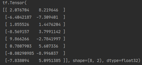

 

4. Define model

w = tf.Variable(tf.random.normal(w0.shape))
b = tf.Variable(tf.zeros_like(b0, dtype=tf.float32))


# Define model
class LinearRegression:
    # Forward propagation
    def __call__(self, x):
        return x @ w + b

    # loss function 
    def loss_func(self, y_true, y_pred):
        return tf.reduce_mean((y_true - y_pred) ** 2 / 2)


model = LinearRegression()

Description:_ call_ Is a special method. Once defined, an instance of a class can become a callable object.

5. Training model

(1) Define train_step completes the gradient calculation and parameter update of each step

(2) During the training process, it is still obvious when using autograph for acceleration, which can be compared and observed.

@tf.function
def train_step(model, features, labels):
    with tf.GradientTape() as tape:
        predictions = model(features)
        loss = model.loss_func(labels, predictions)
    # Back propagation gradient
    dloss_lw, dloss_db = tape.gradient(loss, [w, b])
    # Gradient descent algorithm updating parameters
    w.assign(w - 0.001 * dloss_lw)
    b.assign(b - 0.001 * dloss_db)
    return loss

def train_model(model,epochs):
    for epoch in tf.range(1,epochs+1):
        for features, labels in data_iter(X,Y,10):
            loss = train_step(model,features,labels)

        if epoch%50==0:
            printbar()
            tf.print("epoch =",epoch,"loss = ",loss)
            tf.print("w =",w)
            tf.print("b =",b)

train_model(model,epochs = 200)

(3) Result visualization

# Result visualization
plt.figure(figsize=(12, 5))
ax1 = plt.subplot(121)
ax1.scatter(X[:, 0], Y[:, 0], c="b", label="samples")
ax1.plot(X[:, 0], w[0] * X[:, 0] + b[0], "-r", linewidth=5.0, label="model")
ax1.legend()
plt.xlabel("x1")
plt.ylabel("y", rotation=0)

ax2 = plt.subplot(122)
ax2.scatter(X[:, 1], Y[:, 0], c="g", label="samples")
ax2.plot(X[:, 1], w[1] * X[:, 1] + b[0], "-r", linewidth=5.0, label="model")
plt.xlabel("x2")
plt.ylabel("y", rotation=0)

plt.show()