1, Business background
This experiment will use the time depth learning technology to reconstruct the image with super-resolution. The designed technology includes convolution neural network, generation countermeasure network, residual network and so on.
2, Development environment
This experiment uses "Microsoft Visual Studio", "VS Tools for AI" and other development components, and involves "TensorFlow", "NumPy", "scipy. misc", "PIL.image" and other frameworks and libraries, in which "scipy. misc" and "PIL.image" are used for image processing. This experiment also needs "NVIDIA GPU" driver, "CUDA" and "cuDNN".
See "VS Tools for AI" for detailed environment configuration methods Official documents.
After configuring the environment, enter "Microsoft Visual Studio". The 2017 version is used in this experiment. Click "file", "new", "project", then select "general Python application" in "AI tools", set the project name to "image super resolution", and click "OK" to create the project.
Subsequently, double-click image-super-resolution.sln to enter the project.
3, Data exploration
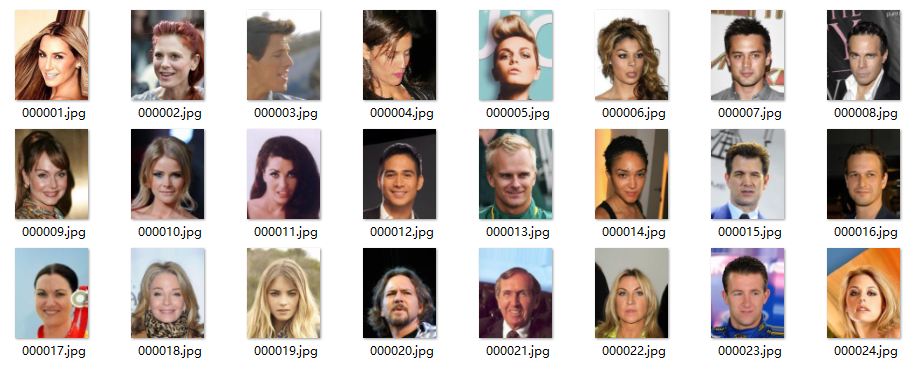
The data of this experiment can be selected from various common data sets in CV field. The experiment will take CelebA data set as an example. CelebA is the face recognition data opened by the Chinese University of Hong Kong, including 202599 pictures of 10177 celebrities, with 5 location markers and 40 attribute markers. It can be used as a data set for face detection, face attribute recognition, face location and other tasks. Datasets are available in Google Drive Download in, details can be found in Official website View in. This experiment uses img in this data set_ align_ celeba. Zip file, the first 10661 pictures are selected, and each picture is adjusted to the size of 219x178 according to the position of the portrait's eyes. The decompressed image is shown in Figure 1.
This experiment needs to get the low resolution images of the image in Figure 1, and promote these low resolution images to high-resolution images through deep learning. Finally, compare them with the original image in Figure 1 to see the effect of the model.
In the problem of image super-resolution, any image data can be selected theoretically. At that time, according to experience, the image with more detailed texture will have better effect, and the PNG image with lossless compression format has better effect than the JPG image.
4, Data preprocessing
The data preprocessing of this experiment needs to organize the original image in Figure 1 into the corresponding input and output of neural network, and enhance the input data. Before preprocessing, move the last five images to a new folder as test images and the rest as training images.
4.1 image size adjustment
The size of the element image in Figure 1 is 219x178. In order to improve the experimental efficiency and effect, first adjust the training and test image to the size of 128x128. Note that the experiment does not directly use the "resize" function, because the down sampling of the "resize" function will reduce the resolution of the image. In the experiment, the "crop" function is used to cut the image in the middle, The last cropped image is persisted.
4.2 loading data
In the experiment, TensorFlow's Dataset API is used, which encapsulates the dataset in a high level, and can perform batch loading, preprocessing, batch reading, shuffle, prefetch and other operations on the data. Note that the prefetch operation requires memory. If the memory is insufficient, prefetch is not required; Because the subsequent network structure of this experiment is deep, there are quite high requirements for video memory. The batch size here is only set to 30. If the video memory is enough or insufficient, it can be adjusted appropriately. This part of the code is shown below.
def load_data(data_dir, training=False):
    filenames = tf.gfile.ListDirectory(data_dir)
    filenames = [os.path.join(data_dir, f) for f in filenames]
    random.shuffle(filenames)

    image_count = len(filenames)

    image_ds = tf.data.Dataset.from_tensor_slices(filenames)
    image_ds = image_ds.map(lambda image_path: preprocess_image(image_path, training=training))

    BATCH_SIZE = 30
    image_ds = image_ds.batch(BATCH_SIZE)

    # image_ds = image_ds.prefetch(buffer_size=400)

    return image_ds
4.3 image preprocessing
In image processing, the image is often enhanced before it is input into the network. There are two main purposes of data enhancement. One is to increase the training data through the random transformation of the image. The other is to make the trained model less affected by irrelevant factors and increase the generalization ability of the image. This section first reads the cropped image in the file; Then, the training image is randomly flipped left and right; And randomly adjust the saturation, brightness, contrast and hue of the image within a certain range; Then normalize the read RGB value to the [- 1, 1] interval; Finally, the bicubic interpolation method is used to sample the image down four times to the size of 32 * 32. The codes in this part are as follows:
def preprocess_image(image_path, training=False):
    image_size = 128
    k_downscale = 4
    downsampled_size = image_size // k_downscale

    image = tf.read_file(image_path)
    image = tf.image.decode_jpeg(image, channels=3)

    if training:    # If the effect is not good, this part of the enhancement can be ignored
        image = tf.image.random_flip_left_right(image)

        image = tf.image.random_saturation(image, 0.95, 1.05)  # saturation
        image = tf.image.random_brightness(image, 0.05)  # brightness
        image = tf.image.random_contrast(image, 0.95, 1.05)  # contrast ratio
        image = tf.image.random_hue(image, 0.05)  # Hue

    label = (tf.cast(image, tf.float32) - 127.5) / 127.5  # normalize to [-1,1] range

    feature = tf.image.resize_images(image, [downsampled_size, downsampled_size], tf.image.ResizeMethod.BICUBIC)
    feature = (tf.cast(feature, tf.float32) - 127.5) / 127.5  # normalize to [-1,1] range

    # if training:
    #     feature = feature + tf.random.normal(feature.get_shape(), stddev=0.03)

    return feature, label
4.4 persistence test data
After pre-processing, the experiment will persist the characteristics and label data of the test set locally, so as to compare with the output of the model in subsequent training. This part of the code is as follows:
def save_feature_label(train_log_dir, test_image_ds):
    feature_batch, label_batch = next(iter(test_image_ds))

    feature_dir = train_log_dir + '0_feature/'
    label_dir = train_log_dir + '0_label/'

    delete_or_makedir(feature_dir)
    delete_or_makedir(label_dir)

    for i, feature in enumerate(feature_batch):
        if i > 5:
            break
        misc.imsave(feature_dir + '{:02d}.png'.format(i), feature)

    for i, label in enumerate(label_batch):
        if i > 5:
            break
        misc.imsave(label_dir + '{:02d}.png'.format(i), label)
5, Model design
This experiment will use the combination of GAN, CNN and ResNet to build a super-resolution model. This section will first introduce the residual block and the up sampled pixel shuffle used in the generator of GAN, then introduce the generator and discriminator in GAN respectively, and finally introduce the training process of the model.
5.1 residual block
The residual network introduces the design of residual block, as shown in Figure 2. The input of the residual block is x, and the output of the normal model design is the output F(x) of the two-layer neural network. The residual block adds the input x to the output F(x) of the two layers, and the result H(x) is the output of the residual block. This design achieves the purpose of the previous hypothesis. The goal of training is to make the residual F(x)=H(x)-x close to 0, that is, H(x) and X approximate as much as possible. With the deepening of the network level, this design ensures that the accuracy of the network will not decline in the subsequent level.
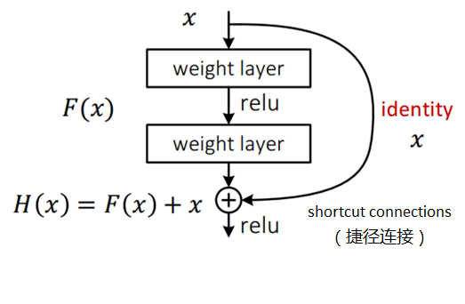
In the implementation of this experiment, the weight layer in the residual block in Figure 2 will be a convolution layer with 64 feature map outputs, convolution kernel size of 3 * 3 and step size of 1, and a Batch Normalization layer is set, and the Relu activation function is also changed to PRelu. The code is as follows:
class _IdentityBlock(tf.keras.Model):
    def __init__(self, filter, stride, data_format):
        super(_IdentityBlock, self).__init__(name='')

        bn_axis = 1 if data_format == 'channels_first' else 3

        self.conv2a = tf.keras.layers.Conv2D(
            filter, (3, 3), strides=stride, data_format=data_format, padding='same', use_bias=False)
        # self.bn2a = tf.keras.layers.BatchNormalization(axis=bn_axis)
        self.prelu2a = tf.keras.layers.PReLU(shared_axes=[1, 2])

        self.conv2b = tf.keras.layers.Conv2D(
            filter, (3, 3), strides=stride, data_format=data_format, padding='same', use_bias=False)
        # self.bn2b = tf.keras.layers.BatchNormalization(axis=bn_axis)

    def call(self, input_tensor):
        x = self.conv2a(input_tensor)
        # x = self.bn2a(x)

        x = self.prelu2a(x)
        x = self.conv2b(x)
        # x = self.bn2b(x)

        x = x + input_tensor
        return x
5.2 upper sampling PixelShuffler
The goal of this experiment is to super-resolution 32x32 low resolution image to 128x128. Therefore, the model inevitably needs up sampling. In the model design stage, the experiment includes the conv2dtransform method, which is deconvolution, that is, the inverse of convolution operation, but the experimental results show that this method will cause very obvious noise pixels; The second upsampling method is TensorFlow UpSampling2D + Conv2D, which is a common inverse operation of max pooling in CNN. The experimental results show that this method loses more information and the experimental effect is poor. This paper finally selects pixel shuffle as the up sampling method. The pixel shuffle operation is shown in Figure 3. For the low-resolution image input as H*W, firstly, r^2 feature images (r is the up sampling factor, i.e. the magnification of the image) are obtained through convolution operation, in which the size of the feature image is consistent with that of the low-resolution image, and then the high-resolution image is obtained through periodic shuffling.
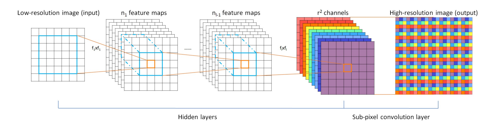
In this experiment, the operation of the convolution part is put into the GAN generator. The following code shows how to select the period on the r^2 feature map to obtain the target high-resolution image output.
def pixelShuffler(inputs, scale=2):
    size = tf.shape(inputs)
    batch_size = size[0]
    h = size[1]
    w = size[2]
    c = inputs.get_shape().as_list()[-1]

    # Get the target channel size
    channel_target = c // (scale * scale)
    channel_factor = c // channel_target

    shape_1 = [batch_size, h, w, channel_factor // scale, channel_factor // scale]
    shape_2 = [batch_size, h * scale, w * scale, 1]

    # Reshape and transpose for periodic shuffling for each channel
    input_split = tf.split(inputs, channel_target, axis=3)
    output = tf.concat([phaseShift(x, scale, shape_1, shape_2) for x in input_split], axis=3)

    return output

def phaseShift(inputs, scale, shape_1, shape_2):
    # Tackle the condition when the batch is None
    X = tf.reshape(inputs, shape_1)
    X = tf.transpose(X, [0, 1, 3, 2, 4])

    return tf.reshape(X, shape_2)
5.3 generator
The basic model used in this experiment is GAN. In the generator part of GAN, high-resolution model output will be generated from low-resolution input. The code of this part is as follows:
class Generator(tf.keras.Model):
    def __init__(self, data_format='channels_last'):
        super(Generator, self).__init__(name='')

        if data_format == 'channels_first':
            self._input_shape = [-1, 3, 32, 32]
            self.bn_axis = 1
        else:
            assert data_format == 'channels_last'
            self._input_shape = [-1, 32, 32, 3]
            self.bn_axis = 3

        self.conv1 = tf.keras.layers.Conv2D(
            64, kernel_size=9, strides=1, padding='SAME', data_format=data_format)

        self.prelu1 = tf.keras.layers.PReLU(shared_axes=[1, 2])

        self.res_blocks = [_IdentityBlock(64, 1, data_format) for _ in range(16)]

        self.conv2 = tf.keras.layers.Conv2D(
            64, kernel_size=3, strides=1, padding='SAME', data_format=data_format)

        self.upconv1 = tf.keras.layers.Conv2D(
            256, kernel_size=3, strides=1, padding='SAME', data_format=data_format)
        self.prelu2 = tf.keras.layers.PReLU(shared_axes=[1, 2])

        self.upconv2 = tf.keras.layers.Conv2D(
            256, kernel_size=3, strides=1, padding='SAME', data_format=data_format)
        self.prelu3 = tf.keras.layers.PReLU(shared_axes=[1, 2])

        self.conv4 = tf.keras.layers.Conv2D(
            3, kernel_size=9, strides=1, padding='SAME', data_format=data_format)

    def call(self, inputs):
        x = tf.reshape(inputs, self._input_shape)

        x = self.conv1(x)
        x = self.prelu1(x)
        x_start = x

        for i in range(len(self.res_blocks)):
            x = self.res_blocks[i](x)

        x = self.conv2(x)
        x = x + x_start

        x = self.upconv1(x)
        x = pixelShuffler(x)
        x = self.prelu2(x)

        x = self.upconv2(x)
        x = pixelShuffler(x)
        x = self.prelu3(x)

        x = self.conv4(x)
        x = tf.nn.tanh(x)
        return x
5.4 discriminator
The input of the GAN discriminator in this experiment is a 128 * 128 image, and the target output is a Boolean value, that is, to judge whether the input image is a real image or a forged image through the model. The generator designed in this experiment is realized by full convolution network. The code of the discriminator is as follows:
class Discriminator(tf.keras.Model):
    def __init__(self, data_format='channels_last'):
        super(Discriminator, self).__init__(name='')

        if data_format == 'channels_first':
            self._input_shape = [-1, 3, 128, 128]
            self.bn_axis = 1
        else:
            assert data_format == 'channels_last'
            self._input_shape = [-1, 128, 128, 3]
            self.bn_axis = 3

        self.conv1 = tf.keras.layers.Conv2D(
            64, kernel_size=3, strides=1, padding='SAME', data_format=data_format)

        self.conv2 = tf.keras.layers.Conv2D(
            64, kernel_size=3, strides=2, padding='SAME', data_format=data_format)
        # self.bn2 = tf.keras.layers.BatchNormalization(axis=self.bn_axis)

        self.conv3 = tf.keras.layers.Conv2D(
            128, kernel_size=3, strides=1, padding='SAME', data_format=data_format)
        # self.bn3 = tf.keras.layers.BatchNormalization(axis=self.bn_axis)

        self.conv4 = tf.keras.layers.Conv2D(
            128, kernel_size=3, strides=2, padding='SAME', data_format=data_format)
        # self.bn4 = tf.keras.layers.BatchNormalization(axis=self.bn_axis)

        self.conv5 = tf.keras.layers.Conv2D(
            256, kernel_size=3, strides=1, padding='SAME', data_format=data_format)
        # self.bn5 = tf.keras.layers.BatchNormalization(axis=self.bn_axis)

        self.conv6 = tf.keras.layers.Conv2D(
            256, kernel_size=3, strides=2, padding='SAME', data_format=data_format)
        # self.bn6 = tf.keras.layers.BatchNormalization(axis=self.bn_axis)

        self.conv7 = tf.keras.layers.Conv2D(
            512, kernel_size=3, strides=1, padding='SAME', data_format=data_format)
        # self.bn7 = tf.keras.layers.BatchNormalization(axis=self.bn_axis)

        self.conv8 = tf.keras.layers.Conv2D(
            512, kernel_size=3, strides=2, padding='SAME', data_format=data_format)
        # self.bn8 = tf.keras.layers.BatchNormalization(axis=self.bn_axis)

        self.fc1 = tf.keras.layers.Dense(1024)
        self.fc2 = tf.keras.layers.Dense(1)

    def call(self, inputs):
        x = tf.reshape(inputs, self._input_shape)
        x = self.conv1(x)
        x = tf.nn.leaky_relu(x)
        x = self.conv2(x)
        # x = self.bn2(x)
        x = tf.nn.leaky_relu(x)
        x = self.conv3(x)
        # x = self.bn3(x)
        x = tf.nn.leaky_relu(x)
        x = self.conv4(x)
        # x = self.bn4(x)
        x = tf.nn.leaky_relu(x)
        x = self.conv5(x)
        # x = self.bn5(x)
        x = tf.nn.leaky_relu(x)
        x = self.conv6(x)
        # x = self.bn6(x)
        x = tf.nn.leaky_relu(x)
        x = self.conv7(x)
        # x = self.bn7(x)
        x = tf.nn.leaky_relu(x)
        x = self.conv8(x)
        # x = self.bn8(x)
        x = tf.nn.leaky_relu(x)
        x = self.fc1(x)
        x = tf.nn.leaky_relu(x)
        x = self.fc2(x)
        return x
5.5 loss function and optimizer definition
In conventional GAN, the loss function of the generator is against loss, which is defined as generating a data distribution that cannot be distinguished by the discriminator, that is, the probability that the discriminator determines the image generated by the generator as a real image is as high as possible. However, in the super-resolution task, such a loss definition is difficult to help the generator generate images with enough real details. Therefore, this experiment adds additional content loss to the generator. There are two ways to define content loss. One is the classical mean square error loss, that is, the mean square error is calculated directly between the network generated by the generator and the real image. In this way, a high signal-to-noise ratio can be obtained, but the image is missing in high-frequency details. The second content loss is based on the VGG loss based on the ReLU activation layer of the pre trained VGG 19 network, and then the current content loss is calculated by calculating the Euclidean distance between the generated image and the feature representation of the original image.
In this experiment, VGG loss is selected as the content loss, and the final generator loss is defined as the weighted sum of content loss and countermeasure loss. The code of this part is as follows. Note that the VGG 19 network used to calculate content loss is first defined:
def vgg19():
    vgg19 = tf.keras.applications.vgg19.VGG19(include_top=False, weights='imagenet', input_shape=(128, 128, 3))
    vgg19.trainable = False
    for l in vgg19.layers:
        l.trainable = False
    loss_model = tf.keras.Model(inputs=vgg19.input, outputs=vgg19.get_layer('block5_conv4').output)
    loss_model.trainable = False
    return loss_model

def create_g_loss(d_output, g_output, labels, loss_model):
    gene_ce_loss = tf.losses.sigmoid_cross_entropy(tf.ones_like(d_output), d_output)

    vgg_loss = tf.keras.backend.mean(tf.keras.backend.square(loss_model(labels) - loss_model(g_output)))

    # mse_loss = tf.keras.backend.mean(tf.keras.backend.square(labels - g_output))

    g_loss = vgg_loss + 1e-3 * gene_ce_loss
    # g_loss = mse_loss + 1e-3 * gene_ce_loss
    return g_loss
The discriminator loss of this experiment is similar to that of the traditional GAN discriminator. The goal is to judge the forged image generated by the generator as false as possible and the real original image as true as possible. The final discriminator loss is the sum of the two parts. The codes of this part are as follows:
def create_d_loss(disc_real_output, disc_fake_output):
    disc_real_loss = tf.losses.sigmoid_cross_entropy(tf.ones_like(disc_real_output), disc_real_output)

    disc_fake_loss = tf.losses.sigmoid_cross_entropy(tf.zeros_like(disc_fake_output), disc_fake_output)

    disc_loss = tf.add(disc_real_loss, disc_fake_loss)
    return disc_loss
The optimizer selects Adam. beta 1 is set to 0.9, beta 2 is set to 0.999, and epsilon is set to 1e-8 to reduce vibration. The code is as follows:
def create_optimizers():
    g_optimizer = tf.train.AdamOptimizer(learning_rate=1e-4, beta1=0.9, beta2=0.999, epsilon=1e-8)
    d_optimizer = tf.train.AdamOptimizer(learning_rate=1e-4, beta1=0.9, beta2=0.999, epsilon=1e-8)

    return g_optimizer, d_optimizer
5.6 training process
The input and output data of the experiment, the generator and discriminator model and the corresponding optimizer have been defined above. This section will introduce the training process. The experiment will first import the above data, model and discriminator, then define a checkpoint to persist and save the model, and then read the data batch by batch for each step of training. The overall training process is as follows:
def train(train_log_dir, train_image_ds, test_image_ds, epochs, checkpoint_dir):
    generator = isr_model.Generator()
    discriminator = isr_model.Discriminator()
    g_optimizer, d_optimizer = isr_model.create_optimizers()

    checkpoint_prefix = os.path.join(checkpoint_dir, "ckpt")
    checkpoint = tf.train.Checkpoint(g_optimizer=g_optimizer,
                                     d_optimizer=d_optimizer,
                                     generator=generator,
                                     discriminator=discriminator)
    loss_model = isr_util.vgg19()

    for epoch in range(epochs):
        all_g_cost = all_d_cost = 0

        step = 0

        it = iter(train_image_ds)
        while True:
            try:
                image_batch, label_batch = next(it)
                step = step + 1
                g_loss, d_loss = train_step(image_batch, label_batch, loss_model, generator, discriminator,
                                            g_optimizer, d_optimizer)
                all_g_cost = all_g_cost + g_loss
                all_d_cost = all_d_cost + d_loss
            except StopIteration:
                break

        generate_and_save_images(train_log_dir, generator, epoch + 1, test_image_ds)

        # saving (checkpoint) the model every 20 epochs
        if (epoch + 1) % 20 == 0:
            checkpoint.save(file_prefix=checkpoint_prefix)
In each step of training, first obtain the forged high-resolution image through the generator, then calculate the loss of the generator and discriminator respectively, and then update the parameters of the generator and discriminator respectively. Note that the training times of the generator and discriminator are 1:1. The code is as follows:
def train_step(feature, label, loss_model, generator, discriminator, g_optimizer, d_optimizer):
    with tf.GradientTape() as g_tape, tf.GradientTape() as d_tape:
        generated_images = generator(feature)

        real_output = discriminator(label)
        generated_output = discriminator(generated_images)

        g_loss = isr_model.create_g_loss(generated_output, generated_images, label, loss_model)
        d_loss = isr_model.create_d_loss(real_output, generated_output)

    gradients_of_generator = g_tape.gradient(g_loss, generator.variables)
    gradients_of_discriminator = d_tape.gradient(d_loss, discriminator.variables)

    g_optimizer.apply_gradients(zip(gradients_of_generator, generator.variables))
    d_optimizer.apply_gradients(zip(gradients_of_discriminator, discriminator.variables))

    return g_loss, d_loss
6, Experimental evaluation
The evaluation part of this experiment will compare the differences between low resolution images, high-resolution images generated by the model and the original images. The training data of this experiment has 10656 pictures, and the test data is 5 pictures. Due to the experimental evaluation of the improvement effect of image resolution, it is not necessary to divide the training set and test set according to a certain proportion, and the more training data also has better modeling effect. However, it should be noted that according to the current model of this experiment, the required video memory is about 6.8G. If you increase the number of batches, increase the number of convolution feature maps, deepen the network or increase the resolution of the original picture, the video memory will be further increased.
In this experiment, the TensorFlow GPU version is used. The GPU of the experiment is NVIDIA GeForce GTX 1080 with a video memory size of 8G. The super parameters of the current experiment have reached the maximum available video memory of the graphics card. One iteration of the current training set takes about 7-8 minutes, and the training of 20 iterations will last about 2.5 hours. The training loss of the first 60 iterations of this experiment is shown in Figure 4.
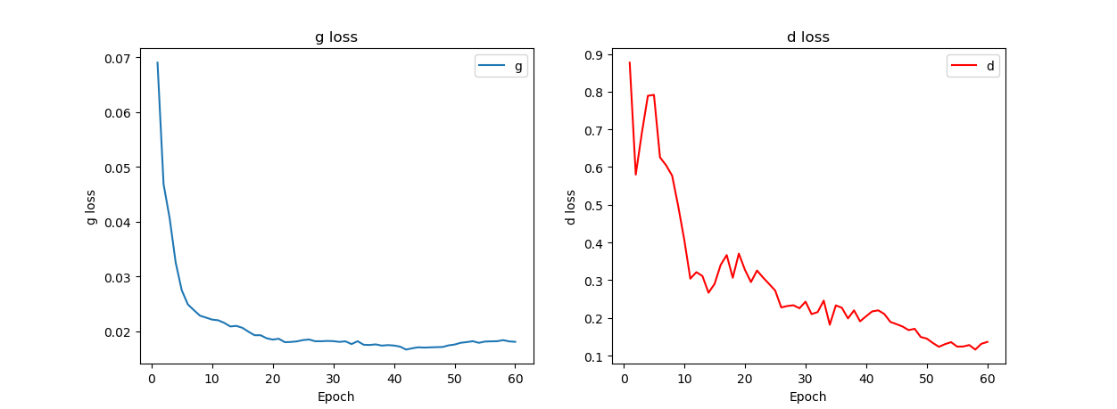
In Figure 4, the loss of the generator decreases in the first 20 iterations of training, fluctuates up and down at 0.02 after 20 to 60 iterations, and the loss further decreases and becomes slow; The loss of the discriminator decreased significantly, but it was noted that there were multiple oscillations. In this experiment, increasing the number of iterations may have a better loss representation.
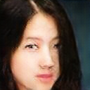
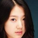
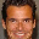
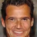
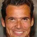
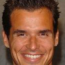
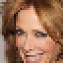
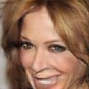
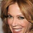
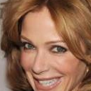
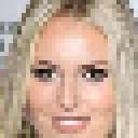
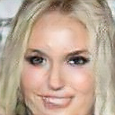
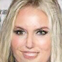
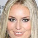
Table 2 shows the performance comparison of the model after 42 iterations and 60 iterations on the test set.
| Input low resolution image | Output after 42 iterations | Output after 60 iterations | Original high resolution image |
|---|---|---|---|
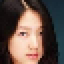 | 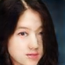 |  |  |
 |  |  |  |
 |  |  |  |
 |  |  |  |
 | 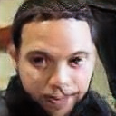 |  |  |
Table 1 shows that the model has a very obvious improvement on the resolution. The details of the first column of low resolution images are very blurred after magnification, while the second column iterates 42 times and the third column iterates 60 times. The image has a clearer outline in some details, such as hair and facial features. However, there is still a gap between the model and the original map, and we can't confuse the false with the true. On the one hand, this is because the experiment is only evaluated on the model after 60 iterations; On the one hand, because the original image is stored in JPG format, it has inherent shortcomings in detail compared with PNG lossless format; Another reason is that this experiment cuts the picture to 128 * 128, which is an expedient measure for video memory. Higher original resolution will have richer detail information. Further increasing the number of iterations, further adjusting parameters, expanding the original size of the image, using the original PNG format image and other methods will lead to a better effect of the final model.
7, Summary
This experiment takes image super-resolution, a hot topic in CV field, as the theme, uses CelebA data set as the experimental data, and constructs a hybrid model of CNN, GAN and ResNet based on GAN as the super-resolution model on the basis of a series of data preprocessing. It has a very obvious effect after 60 times of iterative training. However, due to the objective factors such as GPU computing power and training time, the output of the model is still not perfect compared with the original image. Further experimental ideas include using better machines, increasing the original size of the image, using the original PNG format image, increasing the number of iterations, further adjusting parameters and so on. In addition, GAN training is very difficult and requires patience and some skills to try many times.
notes
For detailed cases, please refer to http://www.biyezuopin.vip
- Written by Zhao Weidong Machine learning case practice Beijing: People's Posts and Telecommunications Press, 2019 (published around June)