1, Spatial data

(1) Definition: spatial data concerns of geographic entities

(2) Classification: raster data model and vector data model are the two most basic ways of spatial data organization in GIS.

    1. Vector Data: as a continuous plane, the map is divided into regularly distributed grids and given different values for each grid. It is commonly used in satellite maps, urban sprawl, etc.

    2. Vector Data: points, lines and faces, which are represented by coordinate axes. Format: shapefile/geojson/DLG, etc.

2, Spatial data visualization -- pattern exploration

(1) Relevance

All things related, but near things are more related than distance things

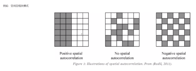    1. Positive spatial autocorrelation, neighbors are the same color as themselves

    2. Similar to random sampling, there is no spatial dependence (autocorrelation)

    3. Negative spatial autocorrelation, the colors of surrounding neighbors are different

(2) Python map visualization - related Library: Folium Library

import folium


m = folium.Map(location=[31.232818,121.475183], zoom_start=12)
# Position as the center point, zoom_start is the map scale size
m


m = folium.Map(
    location=[31.232818,121.475183],
    zoom_start=12,
    tiles = 'http://webrd02.is.autonavi.com/appmaptile?lang=zh_cn&size=1&scale=1&style=7&x={x}&y={y}&z={z}',
    attr = 'default'
)
m


folium.Marker(
    location = [31.143207,121.423575],
    popup = "East China University of Science and Technology",
    icon = folium.Icon(color="red", icon="info-sign"),
).add_to(m)

m

Case: exploratory analysis of visual data of Gaode traffic congestion

(1) Case description: use the real-time congestion index of a city of Gaode traffic big data to find the mode

(2) Basic steps

• capture congestion data and geographic information of a city

• organize geographic information to build geojson and GeoDataFrame

• visual mapping

Step 1: crawl the traffic congestion data and geographic information of a city

※ use the requests library

import requests

header = {"User-Agent" : "Mozilla/5.0 (Windows; u; Windows NT 5.1; zh-CN; rv:1.9.1.6)",
          "Accept" : "text/html, application/xhtml+xml, application/xml; q=0.9, */*; q=0.8",
          "Accept-Language" : "en-us",
          "Connection" : "keep-alive",
          "Accept-Charset" : "GB2312, utf-8; q=0.7, *;q=0.7"}

# city code map
cities_info = requests.get("https://report.amap.com/ajax/getCityInfo.do?", headers = header).json()
city_code_dict = {item["name"]: item["code"] for item in cities_info}



city_code_dict #Form a dictionary, give the city name, and return the city code



# set up city name
city = "Shanghai"




# Webpage: https://report.amap.com/detail.do?city=310000

# to scrape district info
city_content = requests.get('https://report.amap.com/ajax/districtRank.do?linksType=4&cityCode={}'.format(city_code_dict[city]), headers = header).json()

Step 2: organize geographic information to build geojson and GeoDataFrame

※ build geojson (Reference) http://datav.aliyun.com/tools/atlas/index.html)

※ build GeoDataFrame and use geopandas library

# Construct geojson fills in the crawled data
json_data = {'type' : 'FeatureCollection', 'features':[]}
for item in city_content:
    record = dict()
    coords = item["coords"][0][0]
    del item["coords"]
    
    record["type"] = "Feature"
    record["properties"] = item
    coordinates = [[[unit["lon"], unit["lat"]] for unit in coords]]
    record["geometry"] = {"type": "Polygon", "coordinates": coordinates}
    
    json_data["features"].append(record)



json_data    #It's hard to read directly. It's very big



# to check district in amap
m = folium.Map(
    location = [31.143207,121.423575],
    tiles = 'http://webrd02.is.autonavi.com/appmaptile?lang=zh_cn&size=1&scale=1&style=7&x={x}&y={y}&z={z}',
    attr = "default"
)

folium.GeoJson(json_data).add_to(m)
m



import geopandas

geo_data = geopandas.GeoDataFrame.from_features(json_data["features"])
geo_data.crs = "FPSG:4326"

Step 3: draw a visual map——

※ use folium Choropleth() function

m = folium.Map(
    location = [31.143207, 121.423575],
    tiles = 'http://webrd02.is.autonavi.com/appmaptile?lang=zh_cn&size=1&scale=1&style=7&x={x}&y={y}&z={z}',
    attr = "default"
)

folium.Choropleth(
    geo_data = geo_data,
    name = 'Choropleth',
    data = geo_data,
    columns = ["id", "index"],
    key_on = 'feature.properties.id',
    fill_color = 'YlGn',
    fill_opacity = 0.7,  # transparency
    line_opacity = 0.2,
    legend_name = 'index'
).add_to(m)

folium.LayerControl().add_to(m)
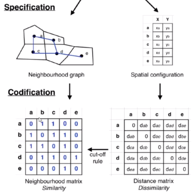
m

3, Topological representation of spatial data -- spatial weight matrix

The modeling of spatial data depends on the spatial information expression of data, that is, their spatial topological relationship.

Generally speaking, in spatial statistical analysis and econometric analysis, spatial weight matrix is used to represent the topology among nodes, regions and individuals.

Since Moran (1948), spatial interaction is often expressed by "weight matrix (W)".

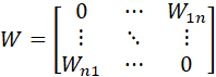
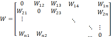
Position in weight matrix Element of Indicates the "proximity" of space units i and j, and the diagonals are 0.

If≠ 0, the spatial unit i is considered as the neighbor of j; Otherwise, it's not.

If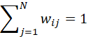, then the weight matrix is called row normalization.  

 

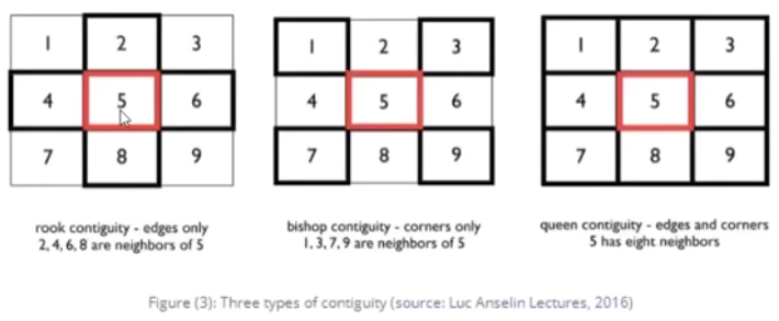
Adjacency classification

4, Spatial autocorrelation test

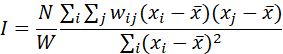
Similar to temporal autocorrelation, spatial data often violates the assumption of independence and has spatial autocorrelation. Moran's l's global and local estimators are commonly used to measure spatial autocorrelation.

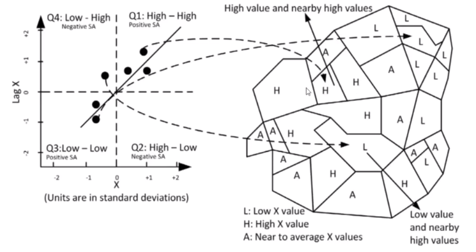
The formula of global Moran's l can be written as

The correlation between Moran's L and spatial pattern is reflected in the figure below. The farther the value of Moran's L is from 0, the more spatial pattern appears.

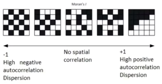
In more detail, the moran diagram can reflect the corresponding relationship between the visual map and the statistics, so as to understand how to identify the spatial pattern through the visual map.

Case: spatial autocorrelation test of urban congestion

(1) The case uses libpysal and esda libraries

(2) Basic steps

• create a spatial weight matrix

• spatial autocorrelation test

Step 1: create a spatial weight matrix

import random
from libpysal.weights import W, Queen, Rook, KNN

# create spatial weight matrix
w_rook = Rook.from_dataframe(geo_data)
w_knn = KNN.from_dataframe(geo_data, k=3)
# Warn: Chongming Island has no neighbors



# see
w_rook.full()



# Normalize
w_rook.transform = 'r'  # Row array planning
w_rook.full()



# to check
district_dict = dict(zip(geo_data.index, geo_data["name"]))
neighbors = dict()
for key in w_rook.neighbors:
    neighbors[district_dict.get(key)] = [district_dict[item] for item in w_rook.neighbors[key]]
neighbors

Step 2: spatial autocorrelation test

from esda.moran import Moran

moran = Moran(geo_data["index"], w_rook)



%matplotlib inline

import matplotlib.pyplot as plt
from splot.esda import plot_moran

plot_moran(moran, zstandard=True, figsize=(10,4))
plt.show



print(f"Moran'I The statistical value of is{moran.I:.4f}, his p Value is{moran.p_sim}. ")



moran_knn = Moran(geo_data["index"], w_knn, transformation="r")
print(f"Moran'I The statistical value of is{moran_knn.I:.4f}, his p Value is{moran_knn.p_sim}. ")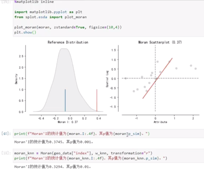

The p value is 0.01, which rejects the original hypothesis and has spatial autocorrelation.

5, Summary and Prospect

(1) Spatial data expansion -- spatio-temporal data

(2) Spatial pattern recognition -- dependence and heterogeneity

(3) Spatial modeling