Basic overview of image retrieval

Since the 1970s, the research on image retrieval has begun. At that time, it is mainly text-based image retrieval technology (TBIR), which uses the way of text description to describe the characteristics of images, such as the author, age, genre and size of paintings.
After the 1990s, image retrieval technology that analyzes and retrieves the content semantics of images, such as image color, texture and layout, namely content-based image retrieval (CBIR) technology. CBIR is a kind of content-based retrieval (CBR). CBR also includes the retrieval technology of dynamic video, audio and other forms of multimedia information.
In terms of retrieval principle, whether it is text-based image retrieval or content-based image retrieval, it mainly includes three aspects: on the one hand, the analysis and transformation of user needs to form questions that can retrieve the index database; On the other hand, collect and process image resources, extract features, analyze and index, and establish image index database; The last aspect is to calculate the similarity between user questions and records in the index database according to the similarity algorithm, extract the records that meet the threshold as the result, and output them in descending order of similarity.
In order to further improve the accuracy of retrieval, many systems combine relevance feedback technology to collect the feedback information of users on the retrieval results, which is more prominent in CBIR, because CBIR realizes the image retrieval process of gradual refinement, and it needs to interact with users continuously in the same retrieval process.

Bag of words model

To understand "Bag of Feature", you must first know "Bag of Words".
"Bag of Words" is an easy to understand strategy in text classification. Generally speaking, if we want to understand the main content of a text, the most effective strategy is to grab the keywords in the text and determine the central idea of the text according to the frequency of keywords. For example, if "iraq" and "terrorism" often appear in a news, we can think that the news should be related to terrorism in iraq. If the key words in a news are "Soviets" and "cuba", we can guess that the news is about the Cold War (see the figure below).

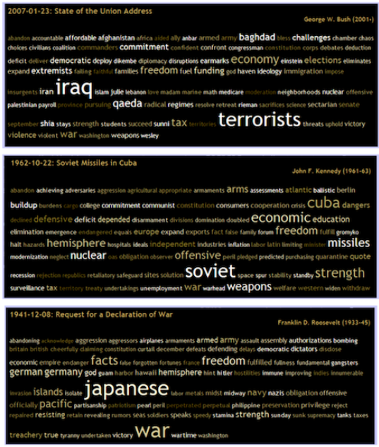
The keywords mentioned here are words in "Bag of words". They are words with high discrimination. According to these words, we can quickly identify the content of the article and quickly classify the article.
The "Bag of Feature" also draws on this idea, but in the image, what we extract is no longer a "word", but the key Feature "Feature" of the image, so the researchers renamed it "Bag of Feature".

Bag of features (BOF)

BOF algorithm flow

1. Collect pictures and extract sift features from the images.
2. Visual words are extracted from each kind of image, and all visual words are collected together
3. Use K-Means algorithm to construct word list.
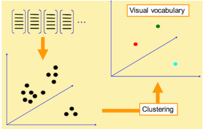
K-Means algorithm is an indirect clustering method based on the similarity measurement between samples. This algorithm takes K as the parameter and divides N objects into K clusters, so that there is high similarity in clusters and low similarity between clusters. According to the distance between the visual word vectors extracted by SIFT, words with similar meaning can be combined by K-Means algorithm as the basic words in the word list
4. The input feature set is quantified according to the visual dictionary, and the input image is transformed into the frequency histogram of visual words.
5. The inverted table of features to images is constructed, and the related images are quickly indexed through the inverted table.
6. Histogram matching is performed according to the index results.

Extracting image features

Features must have high discrimination and meet rotation invariance and size invariance. Therefore, we usually use "SIFT" features. SIFT will extract many feature points from the image, and each feature point is a 128 dimensional vector.

Training dictionary

After extracting features, we will use some clustering algorithms to cluster these feature vectors. The most commonly used clustering algorithm is k-means.
After clustering, we get the dictionary composed of these k vectors. These k vectors have a general expression, which is called visual word.

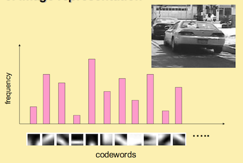
Picture histogram representation

The dictionary trained in the previous step is to quantify the image features in this step. For an image, we can extract a large number of "SIFT" feature points, but these feature points still belong to a low-level expression, which is lack of representativeness. Therefore, the goal of this step is to re extract the high-level features of the image according to the dictionary.

Specifically, for each "SIFT" feature in the image, we can find the most similar visual word in the dictionary. In this way, we can count a k-dimensional histogram to represent the similarity frequency of the "SIFT" feature of the image in the dictionary.

BOF image retrieval

code

Extract SIFT feature points of the image:

# -*- coding: utf-8 -*-
import pickle
from PCV.imagesearch import vocabulary
from PCV.tools.imtools import get_imlist
from PCV.localdescriptors import sift

#Get image list
# imlist = get_imlist('D:/pythonProjects/ImageRetrieval/first500/')
imlist = get_imlist('flowers')
nbr_images = len(imlist)

#Get feature list
featlist = [imlist[i][:-3]+'sift' for i in range(nbr_images)]

#Extract sift features of images under folders
for i in range(nbr_images):
    sift.process_image(imlist[i], featlist[i])

#Generate vocabulary
voc = vocabulary.Vocabulary('ukbenchtest')
voc.train(featlist, 1000, 10)
#Save vocabulary
# saving vocabulary
with open('flowers/vocabulary.pkl', 'wb') as f:
    pickle.dump(voc, f)
print('vocabulary is:', voc.name, voc.nbr_words)

To add an image to the database:

# -*- coding: utf-8 -*-
import pickle
from PCV.imagesearch import imagesearch
from PCV.localdescriptors import sift
from sqlite3 import dbapi2 as sqlite
from PCV.tools.imtools import get_imlist

#Get image list
imlist = get_imlist('flowers')
nbr_images = len(imlist)
#Get feature list
featlist = [imlist[i][:-3]+'sift' for i in range(nbr_images)]

# load vocabulary
#Load vocabulary
with open('flowers/vocabulary.pkl', 'rb') as f:
    voc = pickle.load(f)
#Create index
indx = imagesearch.Indexer('testImaAdd.db',voc)
indx.create_tables()
# go through all images, project features on vocabulary and insert
#Traverse all the images and project their features onto the vocabulary
for i in range(nbr_images)[:500]:
    locs,descr = sift.read_features_from_file(featlist[i])
    indx.add_to_index(imlist[i],descr)
# commit to database
#Submit to database
indx.db_commit()

con = sqlite.connect('testImaAdd.db')
print(con.execute('select count (filename) from imlist').fetchone())
print(con.execute('select * from imlist').fetchone())

Image retrieval test:

# -*- coding: utf-8 -*-
#The position information of image features is not included when using visual words to represent images
import pickle
from PCV.localdescriptors import sift
from PCV.imagesearch import imagesearch
from PCV.geometry import homography
from PCV.tools.imtools import get_imlist

# load image list and vocabulary
#Load image list
imlist = get_imlist('flowers')
nbr_images = len(imlist)
#Load feature list
featlist = [imlist[i][:-3]+'sift' for i in range(nbr_images)]

#Load vocabulary
with open('flowers/vocabulary.pkl', 'rb') as f:
    voc = pickle.load(f)

src = imagesearch.Searcher('testImaAdd.db',voc)# The Searcher class reads the word histogram of the image and executes the query

# index of query image and number of results to return
#Query the image index and the number of images returned by the query
q_ind = 0          # Matched picture subscript
nbr_results = 65  # Dataset size

# regular query
# General query (sort results by Euclidean distance)
res_reg = [w[1] for w in src.query(imlist[q_ind])[:nbr_results]] # Query results
print ('top matches (regular):', res_reg)

# load image features for query image
#Load query image features for matching
q_locs,q_descr = sift.read_features_from_file(featlist[q_ind])
fp = homography.make_homog(q_locs[:,:2].T)

# RANSAC model for homography fitting
#The randac model is used for fitting
model = homography.RansacModel()
rank = {}
# load image features for result
#Load features of candidate images
for ndx in res_reg[1:]:
    try:
        locs,descr = sift.read_features_from_file(featlist[ndx])  # because 'ndx' is a rowid of the DB that starts at 1
    except:
        continue
#get matches
    matches = sift.match(q_descr,descr)
    ind = matches.nonzero()[0]
    ind2 = matches[ind]
    tp = homography.make_homog(locs[:,:2].T)
    # compute homography, count inliers. if not enough matches return empty list
    # Calculate homography matrix
    try:
        H,inliers = homography.H_from_ransac(fp[:,ind],tp[:,ind2],model,match_theshold=4)
    except:
        inliers = []
    # store inlier count
    rank[ndx] = len(inliers)

# sort dictionary to get the most inliers first
# Sorting the dictionary can get the query results after rearrangement
sorted_rank = sorted(rank.items(), key=lambda t: t[1], reverse=True)
res_geom = [res_reg[0]]+[s[0] for s in sorted_rank]
print ('top matches (homography):', res_geom)

# Display query results
imagesearch.plot_results(src,res_reg[:6]) #General query
imagesearch.plot_results(src,res_geom[:6]) #Results after rearrangement

Operation results

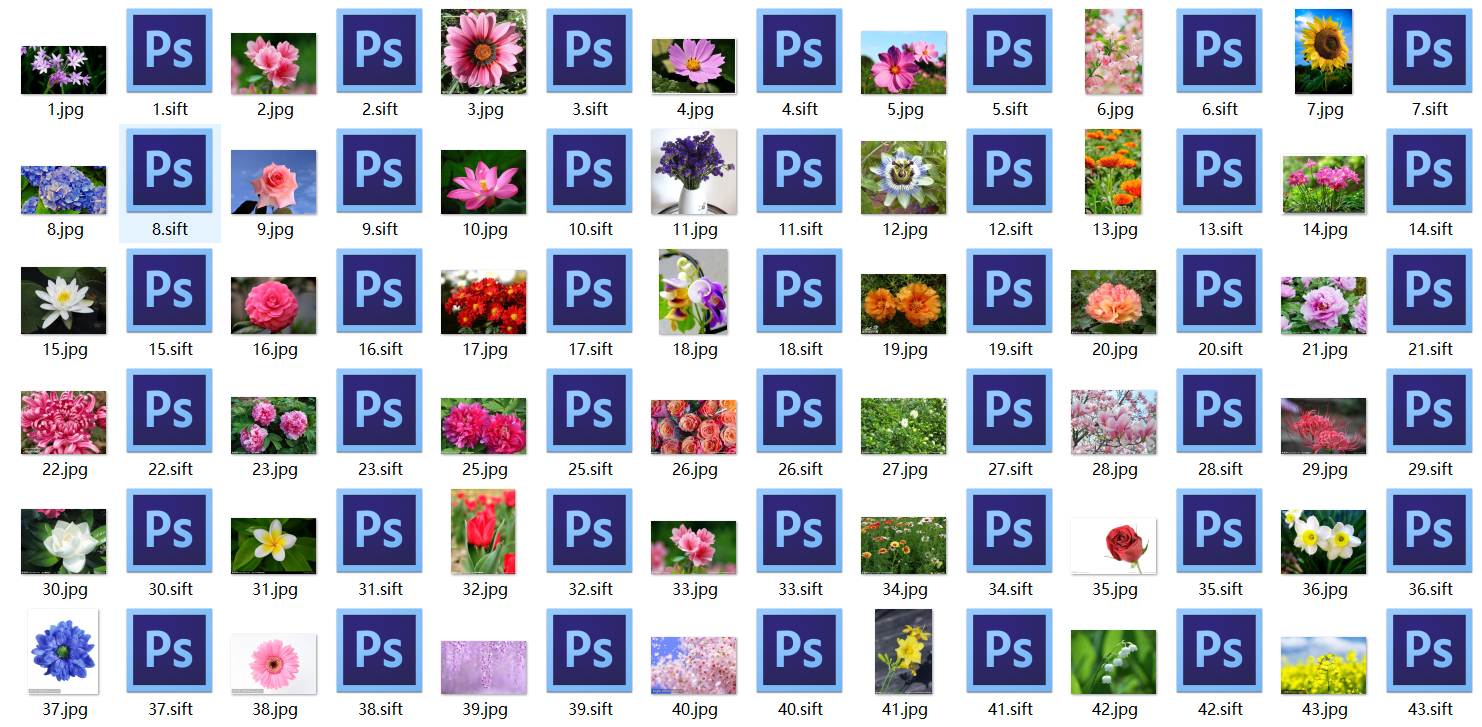
Training set 65 pictures:

Retrieved pictures:

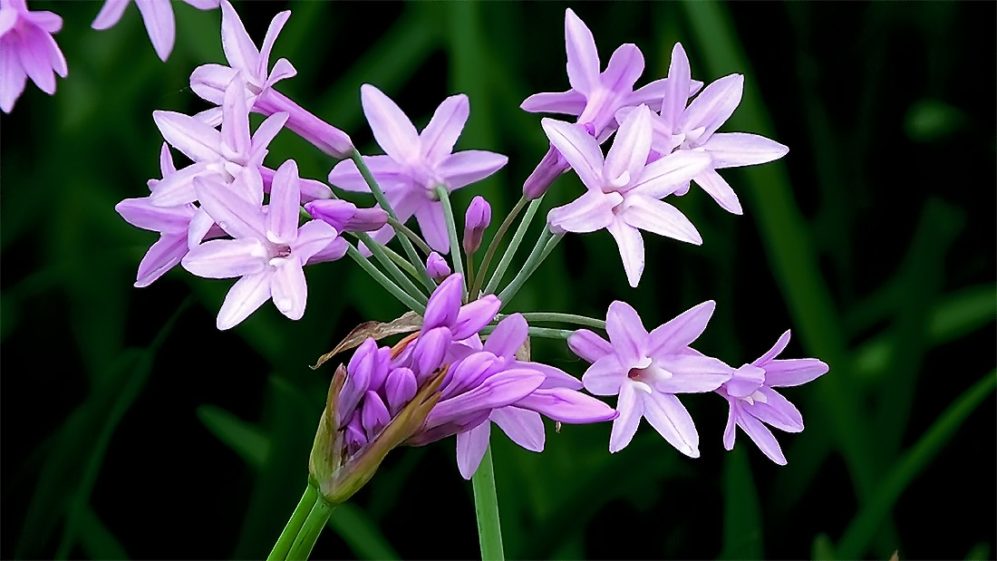
Results of general query:

Result of rearrangement:

Result analysis:
It can be seen from the results that the retrieved 2 and 4 pictures are similar to the input pictures in shape, texture and color. Pictures 1, 3 and 5 are similar in shape and texture, but different in color. From 1 to 4, they are sorted according to the most similar. The rearranged image has changed, but the second similar image actually looks different from the input image.
According to the experimental process, some problems are also found. For a large number of data, the huge input matrix will lead to memory overflow and low efficiency. If the dictionary is too large, the words will lack generality, be sensitive to noise and have a large amount of calculation. The key is the high dimension of the image after projection; If the dictionary is too small, the word discrimination performance is poor, and the similar target features cannot be expressed.
Reference 1