Crawling the data information about python position in the pull net, and storing the crawling data into various csv files, then cleaning the data of the relevant fields in the csv file, and making further analysis on the data visualization, including histogram display, histogram display, word cloud display, etc. according to the visualization data, the rest of the analysis and display readers can play and expand by themselves Including all kinds of analysis and different storage methods.....
1, Crawling and analyzing dependent packages
- Python version: Python 3.6
- requests: Download Web page
- math: round up
- time: pause process
- pandas: data analysis and saving as csv file
- matplotlib: Drawing
- pyecharts: Drawing
- statsmodels: statistical modeling
- wordcloud, scipy, jieba: generate Chinese word cloud
- pylab: set the drawing to display Chinese
In the above installation or use process, the reader may encounter problems such as installation or import failure. Baidu chooses the appropriate version of the dependent package
2, Analyze page structure
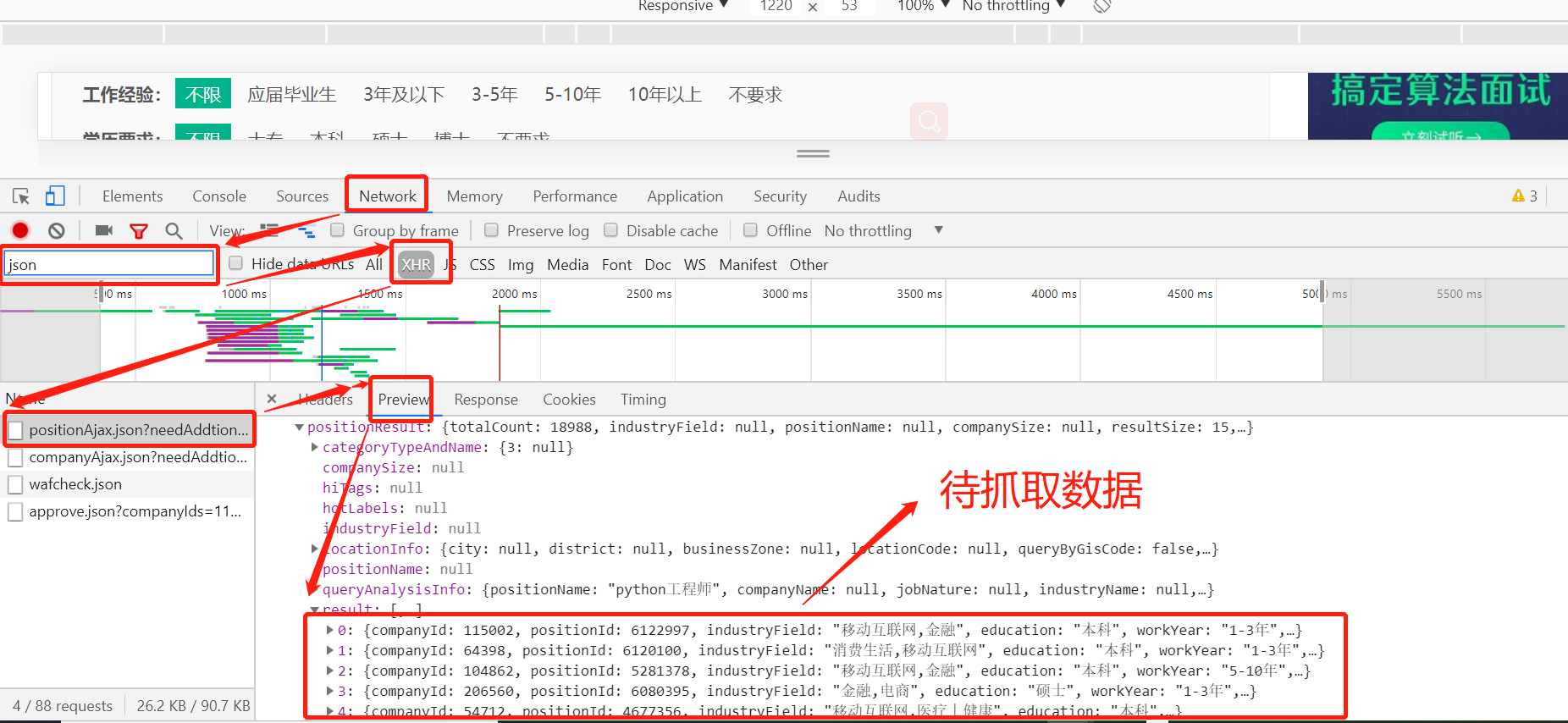
Search 'Python engineer' through Chrome, then right-click check or F12, and use the check function to view the source code of the web page. When we click the next page to observe that the url of the browser's search bar does not change. This is because the anti crawler mechanism is made in the pull-up web, and the position information is not in the source code, but saved in the JSON file, so we download JSON directly, And use the dictionary method to read the data directly. You can get the information about the python position we want,
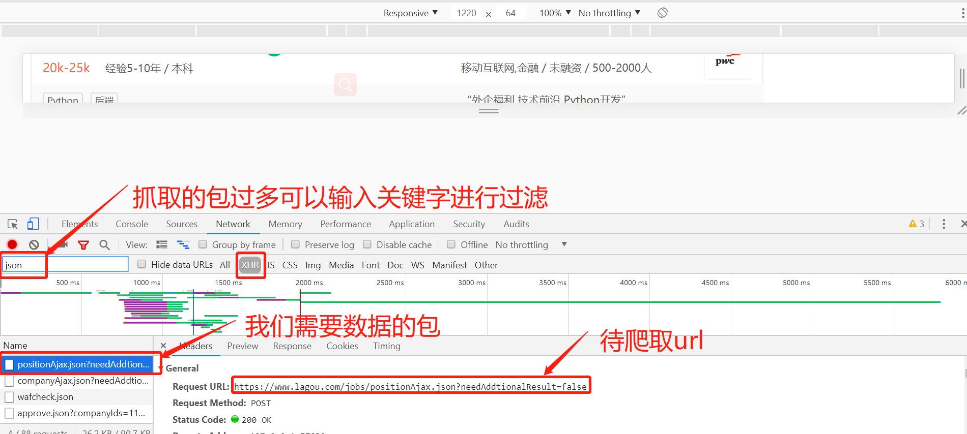
The position information of python engineer to be crawled is as follows:
In order to be able to climb to the data we want, we need to use the program to simulate the browser to view the web page, so we will add the header information in the process of crawling. The header information is also obtained by analyzing the web page. Through the analysis of the web page, we know that the header information of the request, as well as the requested information and the requested method are POST requests, so we can request the url to get it We want to further process the data we want
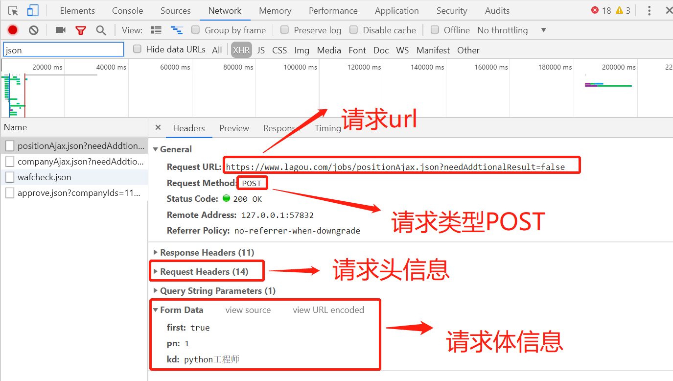
The code of crawling web page information is as follows:
import requests

url = ' https://www.lagou.com/jobs/positionAjax.json?needAddtionalResult=false'


def get_json(url, num):
    """
    //From the specified url, the information in the web page is obtained by carrying the request header and request body through requests,
    :return:
    """
    url1 = 'https://www.lagou.com/jobs/list_python%E5%BC%80%E5%8F%91%E5%B7%A5%E7%A8%8B%E5%B8%88?labelWords=&fromSearch=true&suginput='
    headers = {
        'User-Agent': 'Mozilla/5.0 (Windows NT 10.0; Win64; x64) AppleWebKit/537.36 (KHTML, like Gecko) Chrome/66.0.3359.139 Safari/537.36',
        'Host': 'www.lagou.com',
        'Referer': 'https://www.lagou.com/jobs/list_%E6%95%B0%E6%8D%AE%E5%88%86%E6%9E%90?labelWords=&fromSearch=true&suginput=',
        'X-Anit-Forge-Code': '0',
        'X-Anit-Forge-Token': 'None',
        'X-Requested-With': 'XMLHttpRequest'
    }
    data = {
        'first': 'true',
        'pn': num,
        'kd': 'python engineer'}
    s = requests.Session()
    print('establish session: ', s, '\n\n')
    s.get(url=url1, headers=headers, timeout=3)
    cookie = s.cookies
    print('obtain cookie: ', cookie, '\n\n')
    res = requests.post(url, headers=headers, data=data, cookies=cookie, timeout=3)
    res.raise_for_status()
    res.encoding = 'utf-8'
    page_data = res.json()
    print('Request response result:', page_data, '\n\n')
    return page_data


print(get_json(url, 1))
Through search, we know that each page displays 15 positions, with a maximum of 30 pages. By analyzing the source code of the web page, we can read the total number of positions in JSON, the total number of positions and the number of positions that can be displayed on each page. We can calculate the total number of pages, then use the cycle to crawl by page, and finally summarize the position information and write it into a CSV file
The running result of the program is shown in the figure:
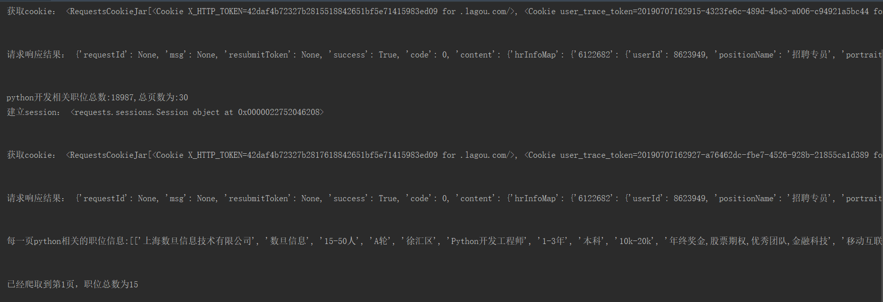
Crawl all python related position information as follows:
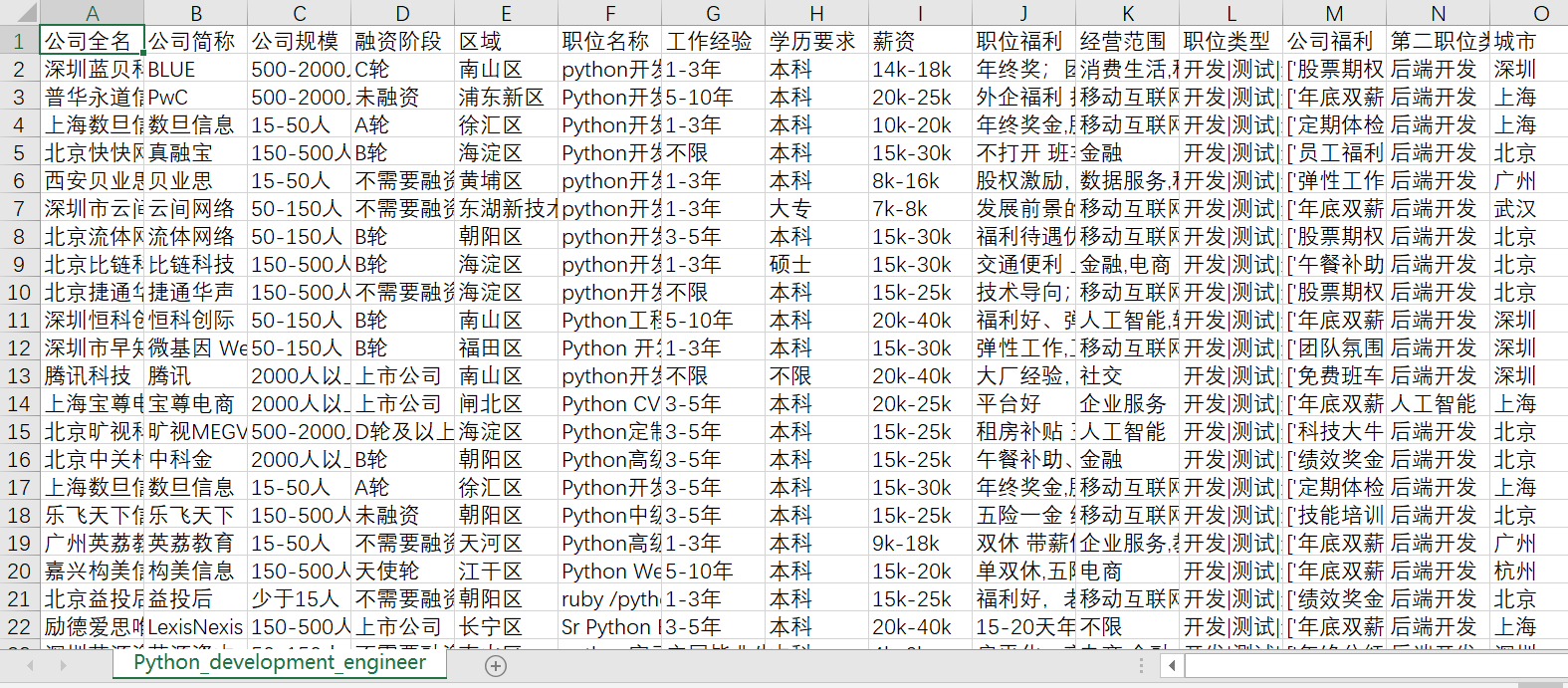
3, Storage after data cleaning
In fact, data cleaning will take up a large part of the work. We only do some simple data analysis here and then store it. There will be 18988 positions related to python input in the network. You can select the fields to be warehoused according to the needs of the work, and further filter some fields. For example, we can remove the positions of interns from the position names, filter the positions of the specified field areas in the areas we specify, take the average value of the field salary, and use the quarter of the minimum value and the difference value as the average value freely according to the needs
import pandas as pd
import matplotlib.pyplot as plt
import statsmodels.api as sm
from wordcloud import WordCloud
from scipy.misc import imread
from imageio import imread
import jieba
from pylab import mpl

# use matplotlib Able to display Chinese
mpl.rcParams['font.sans-serif'] = ['SimHei']  # Specify default font
mpl.rcParams['axes.unicode_minus'] = False  # Resolve save image is negative'-'Questions displayed as squares
#  Read data
df = pd.read_csv('Python_development_engineer.csv', encoding='utf-8')

# Carry out data cleaning and filter out internships
# df.drop(df[df['Job title'].str.contains('internship')].index, inplace=True)
# print(df.describe())


# because csv The characters in the file are in the form of strings. First, regular expressions are used to convert strings into lists, and the mean value of the interval is removed
pattern = '\d+'
# print(df['hands-on background'], '\n\n\n')
# print(df['hands-on background'].str.findall(pattern))
df['Working years'] = df['hands-on background'].str.findall(pattern)
print(type(df['Working years']), '\n\n\n')
avg_work_year = []
count = 0
for i in df['Working years']:
    # print('Working years of each position',i)
    # If the work experience is'unlimited'or'Fresh graduates',Then the matching value is empty,Working life is 0
    if len(i) == 0:
        avg_work_year.append(0)
        # print('nihao')
        count += 1
    # If the match value is a number,Then return the value
    elif len(i) == 1:
        # print('hello world')
        avg_work_year.append(int(''.join(i)))
        count += 1
    # Take the average value if the match is an interval
    else:
        num_list = [int(j) for j in i]
        avg_year = sum(num_list) / 2
        avg_work_year.append(avg_year)
        count += 1
print(count)
df['avg_work_year'] = avg_work_year
# Convert string to list,Minimum salary plus interval value 25%,Close to reality
df['salary'] = df['salary'].str.findall(pattern)
#
avg_salary_list = []
for k in df['salary']:
    int_list = [int(n) for n in k]
    avg_salary = int_list[0] + (int_list[1] - int_list[0]) / 4
    avg_salary_list.append(avg_salary)
df['a monthly salary'] = avg_salary_list
# df.to_csv('python.csv', index=False)
4, Data visualization
The following is a visual display of the data. Only some views are used for visual display. If the reader wants to make some display of other fields and use different view types for display, please play by yourself. Note: see the final completion code for the modules introduced in the following code
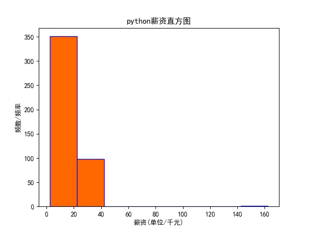
1. Draw frequency histogram of python salary and save it
If we want to see the range and proportion of the general salary of python engineers in the Internet industry, we can use matplotlib library to visualize the data we save in the csv file, and then we can more intuitively see a segment trend of the data
# draw python Frequency histogram of salary and save
plt.hist(df['a monthly salary'],bins=8,facecolor='#ff6700',edgecolor='blue')  # bins Is the default number of bars
plt.xlabel('salary(Company/Thousand yuan)')
plt.ylabel('frequency/frequency')
plt.title('python Salary histogram')
plt.savefig('python Salary distribution.jpg')
plt.show()
The operation results are as follows:
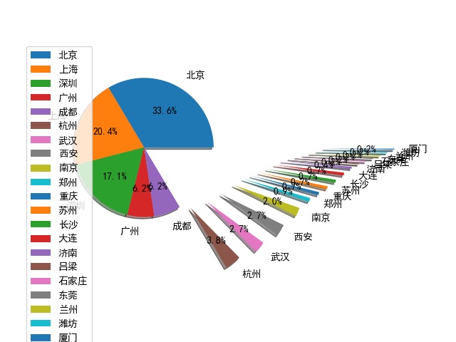
2. Draw pie chart of geographic location of python related positions
Through the geographical python position and geographical location, we can roughly understand which cities the IT industry is mainly concentrated in. In this way, we can choose regions for selective employment and obtain more interview opportunities. The parameters can be adjusted by ourselves or added according to the needs.
# Draw pie chart and save
city = df['city'].value_counts()
print(type(city))
# print(len(city))
label = city.keys()
print(label)
city_list = []
count = 0
n = 1
distance = []
for i in city:

    city_list.append(i)
    print('List length', len(city_list))
    count += 1
    if count > 5:
        n += 0.1
        distance.append(n)
    else:
        distance.append(0)
plt.pie(city_list, labels=label, labeldistance=1.2, autopct='%2.1f%%', pctdistance=0.6, shadow=True, explode=distance)
plt.axis('equal')  # Make the pie a positive circle
plt.legend(loc='upper left', bbox_to_anchor=(-0.1, 1))
plt.savefig('python Geographical location map.jpg')
plt.show()
The operation results are as follows:
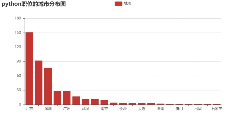
3. Drawing histogram of city distribution based on pyechart
pycharts is the echarts interface that calls Baidu based on js in python. It can also perform various visual operations on data, and display more data in visual graphics. It can refer to echarts official website: https://www.echartsjs.com/ The official website of echarts provides various examples for our reference, such as line chart, histogram, pie chart, path chart, tree chart, etc. the documents based on pyecharts can refer to the following official website: https://pyecharts.org/#/ For more usage, you can also use Baidu network resources by yourself
city = df['city'].value_counts()
print(type(city))
print(city)
# print(len(city))

keys = city.index  # Equivalent to keys = city.keys()
values = city.values
from pyecharts import Bar

bar = Bar("python City map of positions")
bar.add("city", keys, values)
bar.print_echarts_options()  # This line is only for printing configuration items, which is convenient for debugging
bar.render(path='a.html')
The operation results are as follows:
4. Drawing word cloud related to python benefits
Word cloud image, also known as word cloud, is a visual highlight of keywords with high frequency in text data, forming a "keyword rendering" color image similar to cloud, thus filtering out a large number of text information, so that people can understand the main meaning of text data at a glance. Use the jieba segmentation and word cloud to generate the world cloud (customizable background). Here is a word cloud display of the benefits of python related positions, which can more intuitively see where the benefits of most companies are concentrated
# Draw the word cloud of welfare treatment
text = ''
for line in df['Company benefits']:
    if len(eval(line)) == 0:
        continue
    else:
        for word in eval(line):
            # print(word)
            text += word

cut_word = ','.join(jieba.cut(text))
word_background = imread('princess.jpg')
cloud = WordCloud(
    font_path=r'C:\Windows\Fonts\simfang.ttf',
    background_color='black',
    mask=word_background,
    max_words=500,
    max_font_size=100,
    width=400,
    height=800

)
word_cloud = cloud.generate(cut_word)
word_cloud.to_file('Benefits and benefits.png')
plt.imshow(word_cloud)
plt.axis('off')
plt.show()
The operation results are as follows:

5, Crawler and visual complete code
The complete code is below. The code can be tested and run normally. Interested partners can try and understand the usage methods. If the operation or module installation fails, you can leave a message in the comment area. Let's solve it together
If you think it's helpful to you, you can like it. You need to explain the source of the original content reprint!!!
1. Crawler full code
In order to prevent us from frequently requesting a website to be restricted by ip, we choose to sleep for a period of time after crawling each page. Of course, you can also use proxy and other ways to realize it
import requests
import math
import time
import pandas as pd


def get_json(url, num):
    """
    //From the specified url, the information in the web page is obtained by carrying the request header and request body through requests,
    :return:
    """
    url1 = 'https://www.lagou.com/jobs/list_python%E5%BC%80%E5%8F%91%E5%B7%A5%E7%A8%8B%E5%B8%88?labelWords=&fromSearch=true&suginput='
    headers = {
        'User-Agent': 'Mozilla/5.0 (Windows NT 10.0; Win64; x64) AppleWebKit/537.36 (KHTML, like Gecko) Chrome/66.0.3359.139 Safari/537.36',
        'Host': 'www.lagou.com',
        'Referer': 'https://www.lagou.com/jobs/list_%E6%95%B0%E6%8D%AE%E5%88%86%E6%9E%90?labelWords=&fromSearch=true&suginput=',
        'X-Anit-Forge-Code': '0',
        'X-Anit-Forge-Token': 'None',
        'X-Requested-With': 'XMLHttpRequest'
    }
    data = {
        'first': 'true',
        'pn': num,
        'kd': 'python engineer'}
    s = requests.Session()
    print('establish session: ', s, '\n\n')
    s.get(url=url1, headers=headers, timeout=3)
    cookie = s.cookies
    print('obtain cookie: ', cookie, '\n\n')
    res = requests.post(url, headers=headers, data=data, cookies=cookie, timeout=3)
    res.raise_for_status()
    res.encoding = 'utf-8'
    page_data = res.json()
    print('Request response result:', page_data, '\n\n')
    return page_data


def get_page_num(count):
    """
    //Calculate the number of pages to be grabbed. By entering keyword information in the pull-up screen, you can find that up to 30 pages of information are displayed, and up to 15 position information are displayed on each page
    :return:
    """
    page_num = math.ceil(count / 15)
    if page_num > 30:
        return 30
    else:
        return page_num


def get_page_info(jobs_list):
    """
    //Get a position
    :param jobs_list:
    :return:
    """
    page_info_list = []
    for i in jobs_list:  # Cycle all position information on each page
        job_info = []
        job_info.append(i['companyFullName'])
        job_info.append(i['companyShortName'])
        job_info.append(i['companySize'])
        job_info.append(i['financeStage'])
        job_info.append(i['district'])
        job_info.append(i['positionName'])
        job_info.append(i['workYear'])
        job_info.append(i['education'])
        job_info.append(i['salary'])
        job_info.append(i['positionAdvantage'])
        job_info.append(i['industryField'])
        job_info.append(i['firstType'])
        job_info.append(i['companyLabelList'])
        job_info.append(i['secondType'])
        job_info.append(i['city'])
        page_info_list.append(job_info)
    return page_info_list


def main():
    url = ' https://www.lagou.com/jobs/positionAjax.json?needAddtionalResult=false'
    first_page = get_json(url, 1)
    total_page_count = first_page['content']['positionResult']['totalCount']
    num = get_page_num(total_page_count)
    total_info = []
    time.sleep(10)
    print("python Total number of development related positions:{},The total number of pages is:{}".format(total_page_count, num))
    for num in range(1, num + 1):
        # Get position related information on each page
        page_data = get_json(url, num)  # Get response json
        jobs_list = page_data['content']['positionResult']['result']  # Get all on each page python Relevant position information
        page_info = get_page_info(jobs_list)
        print("Every page python Relevant position information:%s" % page_info, '\n\n')
        total_info += page_info
        print('Has climbed to No{}Page, total positions{}'.format(num, len(total_info)))
        time.sleep(20)
        # Convert total data to data frame Re output,Then write to csv In all kinds of documents
        df = pd.DataFrame(data=total_info,
                          columns=['Full name of company', 'Company abbreviation', 'company size ', 'Financing stage', 'region', 'Job title', 'hands-on background', 'Education requirements', 'salary', 'Position benefits', 'Business scope',
                                   'Position type', 'Company benefits', 'Type of second position', 'city'])
        # df.to_csv('Python_development_engineer.csv', index=False)
        print('python Relevant position information saved')


if __name__ == '__main__':
    main()
2. Visual full code
Data visualization involves the use of matplotlib, jieba, wordcloud, pyecharts, pylab, scipy and other modules. Readers can learn how to use each module and the parameters involved
import pandas as pd
import matplotlib.pyplot as plt
import statsmodels.api as sm
from wordcloud import WordCloud
from scipy.misc import imread
# from imageio import imread
import jieba
from pylab import mpl

# use matplotlib Able to display Chinese
mpl.rcParams['font.sans-serif'] = ['SimHei']  # Specify default font
mpl.rcParams['axes.unicode_minus'] = False  # Resolve save image is negative'-'Questions displayed as squares
#  Read data
df = pd.read_csv('Python_development_engineer.csv', encoding='utf-8')

# Carry out data cleaning and filter out internships
# df.drop(df[df['Job title'].str.contains('internship')].index, inplace=True)
# print(df.describe())


# because csv The characters in the file are in the form of strings. First, regular expressions are used to convert strings into lists, and the mean value of the interval is removed
pattern = '\d+'
# print(df['hands-on background'], '\n\n\n')
# print(df['hands-on background'].str.findall(pattern))
df['Working years'] = df['hands-on background'].str.findall(pattern)
print(type(df['Working years']), '\n\n\n')
avg_work_year = []
count = 0
for i in df['Working years']:
    # print('Working years of each position',i)
    # If the work experience is'unlimited'or'Fresh graduates',Then the matching value is empty,Working life is 0
    if len(i) == 0:
        avg_work_year.append(0)
        # print('nihao')
        count += 1
    # If the match value is a number,Then return the value
    elif len(i) == 1:
        # print('hello world')
        avg_work_year.append(int(''.join(i)))
        count += 1
    # Take the average value if the match is an interval
    else:
        num_list = [int(j) for j in i]
        avg_year = sum(num_list) / 2
        avg_work_year.append(avg_year)
        count += 1
print(count)
df['avg_work_year'] = avg_work_year
# Convert string to list,Minimum salary plus interval value 25%,Close to reality
df['salary'] = df['salary'].str.findall(pattern)
#
avg_salary_list = []
for k in df['salary']:
    int_list = [int(n) for n in k]
    avg_salary = int_list[0] + (int_list[1] - int_list[0]) / 4
    avg_salary_list.append(avg_salary)
df['a monthly salary'] = avg_salary_list
# df.to_csv('python.csv', index=False)


"""1,draw python Frequency histogram of salary and save"""
plt.hist(df['a monthly salary'], bins=8, facecolor='#ff6700', edgecolor='blue')  # bins Is the default number of bars
plt.xlabel('salary(Company/Thousand yuan)')
plt.ylabel('frequency/frequency')
plt.title('python Salary histogram')
plt.savefig('python Salary distribution.jpg')
plt.show()

"""2,Draw pie chart and save"""
city = df['city'].value_counts()
print(type(city))
# print(len(city))
label = city.keys()
print(label)
city_list = []
count = 0
n = 1
distance = []
for i in city:

    city_list.append(i)
    print('List length', len(city_list))
    count += 1
    if count > 5:
        n += 0.1
        distance.append(n)
    else:
        distance.append(0)
plt.pie(city_list, labels=label, labeldistance=1.2, autopct='%2.1f%%', pctdistance=0.6, shadow=True, explode=distance)
plt.axis('equal')  # Make the pie a positive circle
plt.legend(loc='upper left', bbox_to_anchor=(-0.1, 1))
plt.savefig('python Geographical location map.jpg')
plt.show()

"""3,Draw the word cloud of welfare treatment"""
text = ''
for line in df['Company benefits']:
    if len(eval(line)) == 0:
        continue
    else:
        for word in eval(line):
            # print(word)
            text += word

cut_word = ','.join(jieba.cut(text))
word_background = imread('princess.jpg')
cloud = WordCloud(
    font_path=r'C:\Windows\Fonts\simfang.ttf',
    background_color='black',
    mask=word_background,
    max_words=500,
    max_font_size=100,
    width=400,
    height=800

)
word_cloud = cloud.generate(cut_word)
word_cloud.to_file('Benefits and benefits.png')
plt.imshow(word_cloud)
plt.axis('off')
plt.show()

"""4,be based on pyechart Histogram of"""
city = df['city'].value_counts()
print(type(city))
print(city)
# print(len(city))

keys = city.index  # Equivalent to keys = city.keys()
values = city.values
from pyecharts import Bar

bar = Bar("python City map of positions")
bar.add("city", keys, values)
bar.print_echarts_options()  # This line is only for printing configuration items, which is convenient for debugging
bar.render(path='a.html')