1.1 Numpy Infrastructure
NumPy array is a multidimensional array object called ndarray. It consists of two parts:
(1) Actual data
(2) Metadata describing these data
# Multidimensional array ndarray

import numpy as np

ar = np.array([1,2,3,4,5,6,7])
print(ar)          # Output arrays, note the format of the arrays: parentheses, no commas between elements (distinguished from lists)
print(ar.ndim)     # The number of dimensions of the output array (axis number), or rank, is also called rank.
print(ar.shape)    # Dimensions of arrays. For arrays of N rows and m columns, shape s are (n, m)
print(ar.size)     # The total number of elements in an array. For an array of N rows and m columns, the total number of elements is n*m.
print(ar.dtype)    # The type of element in an array is similar to type() (note that type() is a function and. dtype is a method)
print(ar.itemsize) # The byte size of each element in the array is 4 for int32l and 8 for float64.
print(ar.data)     # Buffers that contain actual array elements do not usually need to use this attribute because elements are usually retrieved through the index of the array.
ar   # Interactive output, there will be array (array)

# Basic attributes of arrays
# (1) The dimension of an array is called rank, the rank of a one-dimensional array is 1, and the rank of a two-dimensional array is 2, and so on.
# (2) In NumPy, each linear array is called an axes, and rank actually describes the number of axes:
# For example, a two-dimensional array is equivalent to two one-dimensional arrays, in which each element in the first one-dimensional array is a one-dimensional array.
# So one-dimensional arrays are axes in NumPy. The first axis corresponds to the bottom array, and the second axis is the array in the bottom array.
# The number of axes, rank, is the dimension of the array.
[1 2 3 4 5 6 7]
1
(7,)
7
int64
8
<memory at 0x7ff6cc8c8708>

array([1, 2, 3, 4, 5, 6, 7])
# Create arrays: array() functions, which can be lists, meta-ancestors, arrays, generators, etc. in parentheses

ar1 = np.array(range(10))   # integer
ar2 = np.array([1,2,3.14,4,5])   # float
ar3 = np.array([[1,2,3],('a','b','c')])   # Two-dimensional arrays: nested sequences (lists, meta-ancestors are available)
ar4 = np.array([[1,2,3],('a','b','c','d')])   # Note that the number of nested sequences will not be the same.
print(ar1,type(ar1),ar1.dtype)
print(ar2,type(ar2),ar2.dtype)
print(ar3,ar3.shape,ar3.ndim,ar3.size)     # Two-dimensional array, 6 elements
print(ar4,ar4.shape,ar4.ndim,ar4.size)     # One-dimensional array with two elements
[0 1 2 3 4 5 6 7 8 9] <class 'numpy.ndarray'> int64
[1.   2.   3.14 4.   5.  ] <class 'numpy.ndarray'> float64
[['1' '2' '3']
 ['a' 'b' 'c']] (2, 3) 2 6
[list([1, 2, 3]) ('a', 'b', 'c', 'd')] (2,) 1 2
# Create an array: arange(), similar to range(), that returns the value of a uniform interval within a given interval.

print(np.arange(10))    # Return 0-9, integer
print(np.arange(10.0))  # Return 0.0-9.0, floating-point type
print(np.arange(5,12))  # Return 5-11
print(np.arange(5.0,12,2))  # Return 5.0-12.0 with 2 steps
print(np.arange(10000))  # If the array is too large to print, NumPy automatically skips the central part of the array and prints only the corners:
[0 1 2 3 4 5 6 7 8 9]
[ 0.  1.  2.  3.  4.  5.  6.  7.  8.  9.]
[ 5  6  7  8  9 10 11]
[  5.   7.   9.  11.]
[   0    1    2 ..., 9997 9998 9999]
# Create an array: linspace(): Returns num uniformly spaced samples calculated at intervals [start, stop].

ar1 = np.linspace(2.0, 3.0, num=5)
ar2 = np.linspace(2.0, 3.0, num=5, endpoint=False)
ar3 = np.linspace(2.0, 3.0, num=5, retstep=True)
print(ar1,type(ar1))
print(ar2)
print(ar3,type(ar3))
# numpy.linspace(start, stop, num=50, endpoint=True, retstep=False, dtype=None)
# Start: start value, stop: end value
# num: Sample number generated, default 50
# endpoint: If true, stop is the last sample. Otherwise, it is not included. The default value is True.
# retstep: If true, return (sample, step), where step size is the spacing between samples output is a meta-ancestor containing two elements, the first element is array, and the second is the actual value of step size.
[ 2.    2.25  2.5   2.75  3.  ] <class 'numpy.ndarray'>
[ 2.   2.2  2.4  2.6  2.8]
(array([ 2.  ,  2.25,  2.5 ,  2.75,  3.  ]), 0.25) <class 'tuple'>
# Create arrays: zeros()/zeros_like()/ones()/ones_like()

ar1 = np.zeros(5)
ar2 = np.zeros((2,2), dtype = np.int)
print(ar1,ar1.dtype)
print(ar2,ar2.dtype)
print('------')
# numpy.zeros(shape, dtype=float, order='C'): Returns a new array of given shapes and types, filled with zero.
# shape: Array latitude, more than two-dimensional need (), and the input parameters are integers
# dtype: Data type, default numpy.float64
# order: Does C or Fortran store multidimensional data continuously (in rows or columns) in memory?

ar3 = np.array([list(range(5)),list(range(5,10))])
ar4 = np.zeros_like(ar3)
print(ar3)
print(ar4)
print('------')
# Returns an array of zeros with the same shape and type as the given array, where ar4 creates an array of zeros based on the shape and dtype of ar3

ar5 = np.ones(9)
ar6 = np.ones((2,3,4))
ar7 = np.ones_like(ar3)
print(ar5)
print(ar6)
print(ar7)
# ones()/ones_like() is the same as zeros()/zeros_like(), except that it is filled with 1
[ 0.  0.  0.  0.  0.] float64
[[0 0]
 [0 0]] int32
------
[[0 1 2 3 4]
 [5 6 7 8 9]]
[[0 0 0 0 0]
 [0 0 0 0 0]]
------
[ 1.  1.  1.  1.  1.  1.  1.  1.  1.]
[[[ 1.  1.  1.  1.]
  [ 1.  1.  1.  1.]
  [ 1.  1.  1.  1.]]

 [[ 1.  1.  1.  1.]
  [ 1.  1.  1.  1.]
  [ 1.  1.  1.  1.]]]
[[1 1 1 1 1]
 [1 1 1 1 1]]
# Create an array: eye()

print(np.eye(5))
# Create a square N*N unit matrix with a diagonal value of 1 and the rest of 0
[[ 1.  0.  0.  0.  0.]
 [ 0.  1.  0.  0.  0.]
 [ 0.  0.  1.  0.  0.]
 [ 0.  0.  0.  1.  0.]
 [ 0.  0.  0.  0.  1.]]
Data type of ndarray
bool: Boolean type (True or False) stored in one byte
inti An integer whose size is determined by the platform in which it is located (typically int32 or int64)
int8. One byte size, -128 to 127
int16 integers, -32768 to 32767
int32 integers, -2** 31 to 2** 32-1
int64 integers, -2** 63 to 2** 63 - 1
uint8 unsigned integers, 0 to 255
uint16 unsigned integers, 0 to 65535
uint32 unsigned integers, 0 to 2** 32 - 1
uint64 unsigned integers, 0 to 2** 64 - 1
Float 16 Semi-Precision Floating Points: 16 Bits, Positive and Negative Signs 1 Bit, Index 5 Bits, Accuracy 10 Bits
Float 32 Single Precision Floating Points: 32 Bits, Positive and Negative Signs 1 Bit, Exponential 8 Bits, Accuracy 23 Bits
Float 64 or float: 64 bits, plus or minus sign 1 bit, index 11 bits, precision 52 bits
complex64 Complex, which uses two 32-bit floating-point numbers to represent the real part and the imaginary part, respectively
Complex 128 or complex complex complex, with two 64-bit floating-point numbers representing the real part and the imaginary part, respectively
1.2 Numpy Universal Function
basic operation
# Array shape:.T/.reshape()/.resize()

ar1 = np.arange(10)
ar2 = np.ones((5,2))
print(ar1,'\n',ar1.T)
print(ar2,'\n',ar2.T)
print('------')
# T method: transpose, for example, the original shape is (3,4)/(2,3,4), and the result of transposition is (4,3)/(4,3,2) so the result of one-dimensional array transposition remains unchanged.

ar3 = ar1.reshape(2,5)     # Usage 1: Shape existing arrays directly
ar4 = np.zeros((4,6)).reshape(3,8)   # Usage 2: Change the shape directly after generating the array
ar5 = np.reshape(np.arange(12),(3,4))   # Usage 3: Add arrays within parameters, target shape
print(ar1,'\n',ar3)
print(ar4)
print(ar5)
print('------')
# Numpy. reshape (a, new shape, order='C'): Provide a new shape for an array without changing its data, so the number of elements needs to be consistent!!

ar6 = np.resize(np.arange(5),(3,4))
print(ar6)
# numpy.resize(a, new_shape): Returns a new array of specified shapes that can be filled repeatedly with the required number of elements if necessary.
# Note: T/.reshape()/.resize() all generate new arrays!!!
[0 1 2 3 4 5 6 7 8 9]
 [0 1 2 3 4 5 6 7 8 9]
[[ 1.  1.]
 [ 1.  1.]
 [ 1.  1.]
 [ 1.  1.]
 [ 1.  1.]]
 [[ 1.  1.  1.  1.  1.]
 [ 1.  1.  1.  1.  1.]]
------
[0 1 2 3 4 5 6 7 8 9]
 [[0 1 2 3 4]
 [5 6 7 8 9]]
[[ 0.  0.  0.  0.  0.  0.  0.  0.]
 [ 0.  0.  0.  0.  0.  0.  0.  0.]
 [ 0.  0.  0.  0.  0.  0.  0.  0.]]
[[ 0  1  2  3]
 [ 4  5  6  7]
 [ 8  9 10 11]]
------
[[0 1 2 3]
 [4 0 1 2]
 [3 4 0 1]]
# Replication of arrays

ar1 = np.arange(10)
ar2 = ar1
print(ar2 is ar1)
ar1[2] = 9
print(ar1,ar2)
# Recall python's assignment logic: point to a value generated in memory where ar1 and ar2 point to the same value, so ar1 changes, ar2 changes together

ar3 = ar1.copy()
print(ar3 is ar1)
ar1[0] = 9
print(ar1,ar3)
# copy method generates arrays and complete copies of their data
# Remind again:.T/.reshape()/.resize() are all generating new arrays!!!
True
[0 1 9 3 4 5 6 7 8 9] [0 1 9 3 4 5 6 7 8 9]
False
[9 1 9 3 4 5 6 7 8 9] [0 1 9 3 4 5 6 7 8 9]
# Array type conversion:.astype()

ar1 = np.arange(10,dtype=float)
print(ar1,ar1.dtype)
print('-----')
# Array types can be set at parameter positions

ar2 = ar1.astype(np.int32)
print(ar2,ar2.dtype)
print(ar1,ar1.dtype)
# a.astype(): Converting array types
# Note: Get into the habit of using np.int32 for array type instead of int32 directly
[ 0.  1.  2.  3.  4.  5.  6.  7.  8.  9.] float64
-----
[0 1 2 3 4 5 6 7 8 9] int32
[ 0.  1.  2.  3.  4.  5.  6.  7.  8.  9.] float64
# Array stacking

a = np.arange(5)    # A is a one-dimensional array with five elements
b = np.arange(5,9) # b is a one-dimensional array with four elements
ar1 = np.hstack((a,b))  # Note: ((a,b)), the shape here can be different.
print(a,a.shape)
print(b,b.shape)
print(ar1,ar1.shape)
a = np.array([[1],[2],[3]])   # A is a two-dimensional array, three rows and one column
b = np.array([['a'],['b'],['c']])  # b is a two-dimensional array, three rows and one column
ar2 = np.hstack((a,b))  # Note: ((a,b)), the shape must be the same here.
print(a,a.shape)
print(b,b.shape)
print(ar2,ar2.shape)
print('-----')
# numpy.hstack(tup): Horizontal (column order) stacked array

a = np.arange(5)
b = np.arange(5,10)
ar1 = np.vstack((a,b))
print(a,a.shape)
print(b,b.shape)
print(ar1,ar1.shape)
a = np.array([[1],[2],[3]])
b = np.array([['a'],['b'],['c'],['d']])
ar2 = np.vstack((a,b))  # The shape can be different here.
print(a,a.shape)
print(b,b.shape)
print(ar2,ar2.shape)
print('-----')
# numpy.vstack(tup): Vertical (in column order) stacked array

a = np.arange(5)
b = np.arange(5,10)
ar1 = np.stack((a,b))
ar2 = np.stack((a,b),axis = 1)
print(a,a.shape)
print(b,b.shape)
print(ar1,ar1.shape)
print(ar2,ar2.shape)
# numpy.stack(arrays, axis=0): The sequence of arrays connected along the new axis must have the same shape!
# Explain the meaning of the axis parameter, assuming that two arrays [123] and [456], shape s are (3,0)
# axis=0: [[123] [456], shape is (2,3)
# axis=1: [[14] [25] [36], shape is (3,2)
[0 1 2 3 4] (5,)
[5 6 7 8] (4,)
[0 1 2 3 4 5 6 7 8] (9,)
[[1]
 [2]
 [3]] (3, 1)
[['a']
 ['b']
 ['c']] (3, 1)
[['1' 'a']
 ['2' 'b']
 ['3' 'c']] (3, 2)
-----
[0 1 2 3 4] (5,)
[5 6 7 8 9] (5,)
[[0 1 2 3 4]
 [5 6 7 8 9]] (2, 5)
[[1]
 [2]
 [3]] (3, 1)
[['a']
 ['b']
 ['c']
 ['d']] (4, 1)
[['1']
 ['2']
 ['3']
 ['a']
 ['b']
 ['c']
 ['d']] (7, 1)
-----
[0 1 2 3 4] (5,)
[5 6 7 8 9] (5,)
[[0 1 2 3 4]
 [5 6 7 8 9]] (2, 5)
[[0 5]
 [1 6]
 [2 7]
 [3 8]
 [4 9]] (5, 2)
# Array splitting

ar = np.arange(16).reshape(4,4)
ar1 = np.hsplit(ar,2)
print(ar)
print(ar1,type(ar1))
# numpy.hsplit(ary, indices_or_sections): Splitting the array level (column by column) into multiple subarrays column by column
# The output is a list and the elements in the list are arrays.

ar2 = np.vsplit(ar,4)
print(ar2,type(ar2))
# numpy.vsplit(ary, indices_or_sections):: Divide arrays vertically (in line direction) into multiple subarrays by line
[[ 0  1  2  3]
 [ 4  5  6  7]
 [ 8  9 10 11]
 [12 13 14 15]]
[array([[ 0,  1],
       [ 4,  5],
       [ 8,  9],
       [12, 13]]), array([[ 2,  3],
       [ 6,  7],
       [10, 11],
       [14, 15]])] <class 'list'>
[array([[0, 1, 2, 3]]), array([[4, 5, 6, 7]]), array([[ 8,  9, 10, 11]]), array([[12, 13, 14, 15]])] <class 'list'>
# Array Simple Operations

ar = np.arange(6).reshape(2,3)
print(ar + 10)   # addition
print(ar * 2)   # multiplication
print(1 / (ar+1))  # division
print(ar ** 0.5)  # power
# Operations with scalars

print(ar.mean())  # Average Value
print(ar.max())  # Maximum
print(ar.min())  # Find the Minimum
print(ar.std())  # Calculating standard deviation
print(ar.var())  # Calculating variance
print(ar.sum(), np.sum(ar,axis = 0))  # Sum, np.sum() axis 0, sum by column; axis 1, sum by row
print(np.sort(np.array([1,4,3,2,5,6])))  # sort
# Common Functions
[[10 11 12]
 [13 14 15]]
[[ 0  2  4]
 [ 6  8 10]]
[[ 1.          0.5         0.33333333]
 [ 0.25        0.2         0.16666667]]
[[ 0.          1.          1.41421356]
 [ 1.73205081  2.          2.23606798]]
2.5
5
0
1.70782512766
2.91666666667
15 [3 5 7]
[1 2 3 4 5 6]
1.3 Numpy Index and Slice
Core: Basic Index and Slice/Boolean Index and Slice
# Basic Index and Slice

ar = np.arange(20)
print(ar)
print(ar[4])
print(ar[3:6])
print('-----')
# One-Dimensional Array Index and Slice

ar = np.arange(16).reshape(4,4)
print(ar, 'Array axis number%i' %ar.ndim)   # 4*4 array
print(ar[2],  'Array axis number%i' %ar[2].ndim)  # Slice is an element of the next dimension, so it's a one-dimensional array.
print(ar[2][1]) # Quadratic index to get a value in one-dimensional array
print(ar[1:3],  'Array axis number%i' %ar[1:3].ndim)  # A two-dimensional array consisting of two one-dimensional arrays.
print(ar[2,2])  # Third row, third column, in slice array 10
print(ar[:2,1:])  # 1,2 rows, 2,3,4 columns in slice arrays 2-D arrays
print('-----')
# Two-Dimensional Array Index and Slice

ar = np.arange(8).reshape(2,2,2)
print(ar, 'Array axis number%i' %ar.ndim)   # Array of 2*2*2
print(ar[0],  'Array axis number%i' %ar[0].ndim)  # The first element of the next dimension of a three-dimensional array a two-dimensional array
print(ar[0][0],  'Array axis number%i' %ar[0][0].ndim)  # The first element under the first element of the next dimension of a three-dimensional array a one-dimensional array
print(ar[0][0][1],  'Array axis number%i' %ar[0][0][1].ndim)
# ** Three-dimensional Array Index and Slice
[ 0  1  2  3  4  5  6  7  8  9 10 11 12 13 14 15 16 17 18 19]
4
[3 4 5]
-----
[[ 0  1  2  3]
 [ 4  5  6  7]
 [ 8  9 10 11]
 [12 13 14 15]] Array axis number is 2
 [8910 11] Array axis number is 1
9
[[ 4  5  6  7]
 [8910 11]] Array axis number is 2
10
[[1 2 3]
 [5 6 7]]
-----
[[[0 1]
  [2 3]]

 [[4 5]
  [67]] Array axis number is 3
[[0 1]
 The number of axes of [23]] array is 2
 The number of axes of [0 1] array is 1
 1 Array axis number 0
# Boolean Index and Slice

ar = np.arange(12).reshape(3,4)
i = np.array([True,False,True])
j = np.array([True,True,False,False])
print(ar)
print(i)
print(j)
print(ar[i,:])  # In the first dimension, only True is retained, where the first dimension is line, ar[i,:] = ar[i] (simple writing format)
print(ar[:,j])  # In the second dimension, if ar[:,i] has a warning, because I is three elements, and AR has four elements in the column.
# Boolean Index: Screening with Boolean Matrix

m = ar > 5
print(m)  # Here m is a judgment matrix.
print(ar[m])  # Use m judgment matrix to filter the elements > 5 in ar array key points! The latter pandas judgment principle comes from here.
[[ 0  1  2  3]
 [ 4  5  6  7]
 [ 8  9 10 11]]
[ True False  True]
[ True  True False False]
[[ 0  1  2  3]
 [ 8  9 10 11]]
[[0 1]
 [4 5]
 [8 9]]
[[False False False False]
 [False False  True  True]
 [ True  True  True  True]]
[ 6  7  8  9 10 11]
# Value change and copy of array index and slice

ar = np.arange(10)
print(ar)
ar[5] = 100
ar[7:9] = 200
print(ar)
# When a scalar is assigned to an index/slice, the original array is automatically changed/propagated

ar = np.arange(10)
b = ar.copy()
b[7:9] = 200
print(ar)
print(b)
# copy
[0 1 2 3 4 5 6 7 8 9]
[  0   1   2   3   4 100   6 200 200   9]
[0 1 2 3 4 5 6 7 8 9]
[  0   1   2   3   4   5   6 200 200   9]
1.4 Numpy Random Number
numpy.random contains random samples with multiple probability distributions and is one of the key tools for data analysis.
'''
```python
# generation of random number

samples = np.random.normal(size=(4,4))
print(samples)
# Generate a 4*4 sample value of the standard orthogonal distribution
[[ 0.17875618 -1.19367146 -1.29127688  1.11541622]
 [ 1.48126355 -0.81119863 -0.94187702 -0.13203948]
 [ 0.11418808 -2.34415548  0.17391121  1.4822019 ]
 [ 0.46157021  0.43227682  0.58489093  0.74553395]]
# Numpy. random. Rand (d0, d1,..., dn): generate a random floating point or N-dimensional floating point array between [0, 1] - uniform distribution

import matplotlib.pyplot as plt  # Import matplotlib module for graph aided analysis
% matplotlib inline
# Magic function, automatically generate charts for each run

a = np.random.rand()
print(a,type(a))  # Generate a random floating point number

b = np.random.rand(4)
print(b,type(b))  # Generate one-dimensional arrays of shape 4

c = np.random.rand(2,3)
print(c,type(c))  # Generate a two-dimensional array with a shape of 2*3. Note that this is not ((2,3))

samples1 = np.random.rand(1000)
samples2 = np.random.rand(1000)
plt.scatter(samples1,samples2)
# Generating 1000 uniformly distributed sample values
0.3671245126484347 <class 'float'>
[ 0.95365841  0.45627035  0.71528562  0.98488116] <class 'numpy.ndarray'>
[[ 0.82284657  0.95853197  0.87376954]
 [ 0.53341526  0.17313861  0.18831533]] <class 'numpy.ndarray'>


<matplotlib.collections.PathCollection at 0x7bb52e8>

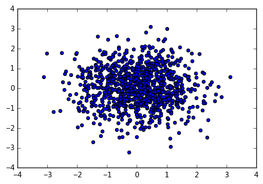
#  Numpy. random. randn (d0, d1,..., dn): Generate a floating-point or N-dimensional floating-point array - Normal distribution

samples1 = np.random.randn(1000)
samples2 = np.random.randn(1000)
plt.scatter(samples1,samples2)
# The parameter usage of randn and rand is the same
# Generate 1000 orthodox sample values
<matplotlib.collections.PathCollection at 0x842ea90>
# numpy.random.randint(low, high=None, size=None, dtype='l'): Generates an array of integers or N-dimensional integers
# If high is not None, take random integers between [low, high], otherwise take random integers between [0, low], and high must be greater than low.
# dtype parameter: only int type

print(np.random.randint(2))
# low=2: Generate a random integer between [0, 2]

print(np.random.randint(2,size=5))
# low=2,size=5: generate five random integers between [0, 2]

print(np.random.randint(2,6,size=5))
# low=2,high=6,size=5: generate five random integers between [2, 6]

print(np.random.randint(2,size=(2,3)))
# Low = 2, size = 2, 3): Generate a 2x3 integer array in the range of [0, 2] random integers

print(np.random.randint(2,6,(2,3)))
# Low = 2, high = 6, size = 2,3): Generate a 2*3 integer array with a range of values: [2,6] Random integers
0
[0 1 1 0 1]
[2 5 2 3 5]
[[0 1 1]
 [1 1 1]]
[[4 4 3]
 [2 3 3]]
1.5 Numpy data input and output
numpy reads / writes array and text data
# Store array data. npy file

import os
os.chdir('C:/Users/Hjx/Desktop/')

ar = np.random.rand(5,5)
print(ar)
np.save('arraydata.npy', ar)
# It can also be directly np.save('C:/Users/Hjx/Desktop/arraydata.npy', ar)
[[ 0.57358458  0.71126411  0.22317828  0.69640773  0.97406015]
 [ 0.83007851  0.63460575  0.37424462  0.49711017  0.42822812]
 [ 0.51354459  0.96671598  0.21427951  0.91429226  0.00393325]
 [ 0.680534    0.31516091  0.79848663  0.35308657  0.21576843]
 [ 0.38634472  0.47153005  0.6457086   0.94983697  0.97670458]]
# Read array data. npy file

ar_load =np.load('arraydata.npy')
print(ar_load)
# Or directly np.load('C:/Users/Hjx/Desktop/arraydata.npy')
[[ 0.57358458  0.71126411  0.22317828  0.69640773  0.97406015]
 [ 0.83007851  0.63460575  0.37424462  0.49711017  0.42822812]
 [ 0.51354459  0.96671598  0.21427951  0.91429226  0.00393325]
 [ 0.680534    0.31516091  0.79848663  0.35308657  0.21576843]
 [ 0.38634472  0.47153005  0.6457086   0.94983697  0.97670458]]
# Store/read text files

ar = np.random.rand(5,5)
np.savetxt('array.txt',ar, delimiter=',')
# np.savetxt(fname, X, fmt='%.18e', delimiter=' ', newline='\n', header='', footer='', comments='# ': Stored as text txt file

ar_loadtxt = np.loadtxt('array.txt', delimiter=',')
print(ar_loadtxt)
# It can also be directly np.loadtxt('C:/Users/Hjx/Desktop/array.txt')
[[ 0.28280684  0.66188985  0.00372083  0.54051044  0.68553963]
 [ 0.9138449   0.37056825  0.62813711  0.83032184  0.70196173]
 [ 0.63438739  0.86552157  0.68294764  0.2959724   0.62337767]
 [ 0.67411154  0.87678919  0.53732168  0.90366896  0.70480366]
 [ 0.00936579  0.32914898  0.30001813  0.66198967  0.04336824]]