In machine learning and deep learning, the input data such as image, sound and text are finally converted into arrays or matrices. How to operate arrays and matrices effectively? Use Numpy. Numpy is a common language for data science and is closely related to PyTorch It is the cornerstone of scientific computing and deep learning, especially for PyTorch. Tensor in PyTorch is very similar to Numpy, which can be easily converted. Mastering Numpy is an important basis for learning PyTorch well.
Why Numpy? Python itself contains lists and arrays, but in deep learning, objects with such structures are not satisfied. Since the elements of the list can be any object, what is saved in the list is the pointer to the object. For example, in order to save a [1,2,3], you need three pointers and three integer objects. For numerical operation, this structure wastes valuable resources such as memory and CPU. As for the array object, it can directly save values, which is similar to the one-dimensional array of C language. However, it does not support multidimensional and is not suitable for numerical operations.
Numpy (Numerical Python) makes up for these shortcomings. Numpy provides two basic objects: ndarray (N-dimensional Array Object) and ufunc (Universal Function Object). ndarray is a multidimensional array that stores a single data type, while ufunc is a function that can process the array.
Main features of Numpy:
- ndarray, a fast space-saving multidimensional array, provides array arithmetic operations and advanced broadcasting functions.
- Use standard mathematical functions to quickly calculate the data of the whole array, and there is no need to write a loop.
- A tool for reading / writing array data on disk and manipulating storage image files.
- Linear algebra, random number generation and Fourier transform.
- Tools for integrating C, C + +, Fortran code.
1. Generate Numpy array
Numpy is an external Python library and is no longer in the standard library. Therefore, when using, you should first import numpy
import numpy as np
After importing Numpy, you can use NP+ Tab key to view the available functions
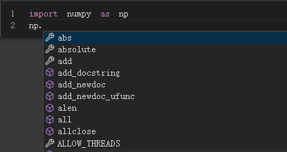
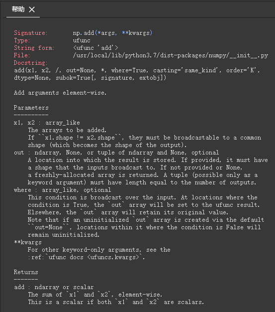
If you are not clear about the use of some of these functions, you can use them in the corresponding function +?, Run again, and you can see the help information on how to use the function.

Numpy encapsulates a new data type ndarray (N-dimensional Array), which is a multi-dimensional array object. The object encapsulates many commonly used mathematical operation functions to facilitate data processing and data analysis. How to generate ndarray? Here are several ways to generate ndarray, such as creating from existing data, creating with random, creating multidimensional arrays with specific shapes, and generating them with rangeand linspace functions.
1.1 create an array from existing data
Directly convert Python basic data types (such as lists, tuples, etc.) to generate ndarray:
1) Convert list to ndarray
import numpy as np

lst1=[3,4,5,6,1,2]
nd1=np.array(lst1)
print(nd1)

print(type(nd1))
Output:
[3 4 5 6 1 2]
<class 'numpy.ndarray'>
2) Convert nested list to multidimensional ndarray
import numpy as np

lst2=[[2,3,4,5],[9,8,7,6]]
nd2=np.array(lst2)
print(nd2)

print(type(nd2))
Output:
[[2 3 4 5]
 [9 8 7 6]]
<class 'numpy.ndarray'>
Replacing the above list with tuples also applies.
1.2 using random module to generate array
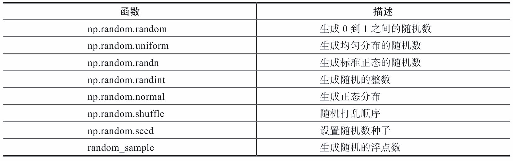
In deep learning, some parameters often need to be initialized. In order to train the model more effectively and improve the performance, some initialization also need to meet certain conditions, such as normal distribution or uniform distribution. Several common methods are introduced here, including NP Random module is a common function.
import numpy as np

nd3=np.random.random([4,4])
print(nd3)

print("nd3 Shape of:",nd3.shape)
Output:
[[0.53403198 0.98447249 0.00533233 0.65173917]
 [0.87977903 0.16099692 0.18023754 0.97709347]
 [0.04435656 0.98775115 0.59948141 0.51385331]
 [0.6364136  0.6397407  0.2583276  0.18612369]]
nd3 Shape of: (4, 4)
nd3 Type: <class 'numpy.ndarray'>
In order to generate the same data each time, specify a random seed, and use the shuffle function to disrupt the generated random number.
import numpy as np

np.random.seed(100)
nd4 = np.random.randn(2,3)
print(nd4)
np.random.shuffle(nd4)
print("Randomly scrambled data:")
print(nd4)
print(type(nd4))
Output:
[[-1.74976547  0.3426804   1.1530358 ]
 [-0.25243604  0.98132079  0.51421884]]
Randomly scrambled data:
[[-1.74976547  0.3426804   1.1530358 ]
 [-0.25243604  0.98132079  0.51421884]]
<class 'numpy.ndarray'>
1.3 creating multidimensional arrays of specific shapes
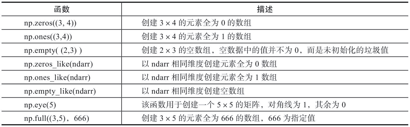
During parameter initialization, it is sometimes necessary to generate some special matrices, such as arrays or matrices with all 0 or 1. At this time, NP zeros,np.ones,np.diag. As follows:
Examples are as follows:
import numpy as np

# Generate a 3x3 matrix with all zeros
nd5 =np.zeros([3, 3])
print(nd5)

#Generate an all-0 matrix with the same shape as nd5
#np.zeros_like(nd5)

# Generate a 3x3 matrix with all 1
nd6 = np.ones([3, 3])
print(nd6)


# Generating a 3rd order identity matrix
nd7 = np.eye(3)
print(nd7)

# Generate third-order diagonal matrix
nd8 = np.diag([1, 2, 3])
print(nd8)
Sometimes it may be necessary to save the generated data temporarily for subsequent use.
import numpy as np

nd9 =np.random.random([5, 5])
np.savetxt(X=nd9, fname='./test1.txt')
nd10 = np.loadtxt('./test1.txt')
print(nd10)
Output:
[[0.87014264 0.06368104 0.62431189 0.52334774 0.56229626]
 [0.00581719 0.30742321 0.95018431 0.12665424 0.07898787]
 [0.31135313 0.63238359 0.69935892 0.64196495 0.92002378]
 [0.29887635 0.56874553 0.17862432 0.5325737  0.64669147]
 [0.14206538 0.58138896 0.47918994 0.38641911 0.44046495]]
1.4 generate array by using range and linspace functions
Range is a function in numpy module. Its format is:
arange([start,] stop[, step,], dtype=None)
Start and stop are used to specify the range, and step is used to set the step size. When generating an ndarray, start defaults to 0, and step can be a decimal. Similar to Python's built-in function range.
import numpy as np

print(np.arange(10))
# [0 1 2 3 4 5 6 7 8 9]

print(np.arange(0, 10))
# [0 1 2 3 4 5 6 7 8 9]

print(np.arange(1, 4, 0.5))
# [1. 1.5 2. 2.5 3. 3.5]

print(np.arange(9, -1, -1))
# [9 8 7 6 5 4 3 2 1 0]
linspace is also a common function in numpy module. Its format is:
np.linspace(start, stop, num=50, endpoint=True, retstep=False, dtype=None, axis=0)
linspace can automatically generate a linear bisection vector according to the specified data range and bisection quantity. The default value of endpoint (including endpoint) is True, and the default value of bisection quantity num is 50. If retstep is set to True, an ndarray with steps is returned.
import numpy as np

print(np.linspace(0,1,10))
#[0.         0.11111111 0.22222222 0.33333333 0.44444444 0.55555556
# 0.66666667 0.77777778 0.88888889 1.
In addition to the range and linspace described above, Numpy also provides the logspace function, which is used in the same way as linspace
import numpy as np

print(np.logspace(0.1,1,10))
#[ 1.25892541  1.58489319  1.99526231  2.51188643  3.16227766  3.98107171
#  5.01187234  6.30957344  7.94328235 10.        ]
2. Get element
The above describes several methods of generating ndarray. After data generation, how to read the required data?
import numpy as np

np.random.seed(2019)
nd11 = np.random.random([10])

#Get the data at the specified location and get the fourth element
nd11[3]

#Intercept a piece of data
nd11[3:6]

#Intercept fixed interval data
nd11[1:6:2]

#Reverse access
nd11[::-2]

#Intercepts data in a region of a multidimensional array
nd12=np.arange(25).reshape([5,5])
nd12[1:3,1:3]

#Intercept the data in a multi-dimensional array whose value is within a value range
nd12[(nd12>3)&(nd12<10)]

#Intercept the specified row in the multidimensional array, such as reading rows 2 and 3
nd12[[1,2]] #Or nd12[1:3,:]

##Intercept the specified column in the multidimensional array, such as reading the 2nd and 3rd columns
nd12[:,1:3]
In addition to specifying the index tag to obtain some elements in the array, it can also be achieved by using some functions, such as random The choice function randomly extracts data from the specified sample.
import numpy as np
from numpy import random as nr

a=np.arange(1,25,dtype=float)
c1=nr.choice(a,size=(3,4)) #size specifies the shape of the output array
c2=nr.choice(a,size=(3,4),replace=False) #replace defaults to True to repeat extraction.
#In the following formula, parameter p specifies the extraction probability corresponding to each element. By default, the probability of each element being extracted is the same.
c3=nr.choice(a,size=(3,4),p=a / np.sum(a))
print("Random repeatable extraction")
print(c1)
print("Random but not repeated extraction")
print(c2)
print("Random but according to institutional probability")
print(c3)
Output:
Random repeatable extraction
[[19.  6. 24. 22.]
 [21. 17. 16.  2.]
 [23. 15. 13. 11.]]
Random but not repeated extraction
[[ 5. 14. 23. 15.]
 [ 8. 24.  6. 18.]
 [13. 10. 21. 11.]]
Random but according to institutional probability
[[19. 21. 18. 11.]
 [10. 21. 23. 19.]
 [18. 19. 11. 20.]]
1.3 Numpy arithmetic operation
Machine learning and deep learning involve a large number of array or matrix operations, which are two common operations. One is the multiplication of corresponding elements, also known as element wise product, and the operator is NP Multiply(), or *. The other is dot product or inner product element, and the operator is NP dot().
1.3.1 multiplication of corresponding elements
Element wise product is the product of corresponding elements in two matrices. np. The multiply function is used to multiply the corresponding elements of the array or matrix. The output is consistent with the size of the multiplied array or matrix. The format is as follows:
multiply(x1, x2, /, out=None, *, where=True, casting='same_kind', order='K', dtype=None, subok=True[, signature, extobj])
The multiplication of the corresponding elements between x1 and x2 complies with the broadcasting rules, which is illustrated by some examples below.
import numpy as np

A = np.array([[1, 2], [-1, 4]])
B = np.array([[2, 0], [3, 4]])
A*B
Output:
array([[ 2,  0],
       [-3, 16]])
Numpy arrays can not only multiply the corresponding elements of the array, but also operate with a single value (or scalar). During operation, each element in numpy array operates with scalar, and broadcast mechanism is used
By extension, after the array passes through some activation functions, the output is consistent with the input shape.
X=np.random.rand(2,3)

def softmoid(x):
  return 1/(1+np.exp(-x))

def relu(x):
  return np.maximum(0,x)

def softmax(x):
  return np.exp(x)/np.sum(np.exp(x))

print("input parameter  X Shape of:",X.shape)
print("Activation function softmoid Output shape:",softmoid(X).shape)
print("Activation function relu Output shape:",relu(X).shape)
print("Activation function softmax Output shape:",softmax(X).shape)
Output:
input parameter  X Shape of: (2, 3)
Activation function softmoid Output shape: (2, 3)
Activation function relu Output shape: (2, 3)
Activation function softmax Output shape: (2, 3)
1.3.2 point product operation
Dot Product operation is also called inner product, and NP is used in Numpy Dot indicates, and its general format is:
numpy.dot(a, b, out=None)
import numpy as np

X1=np.array([[1,2],[3,4]])
X2=np.array([[5,6,7],[8,9,10]])
X3=np.dot(X1,X2)
print(X3)
Output:
[[21 24 27]
 [47 54 61]]
Matrix X1 and matrix x2 perform dot product operation, in which the number of elements of the corresponding dimensions of X1 and X2 (i.e. the second dimension of X1 and the first dimension of x2) must be consistent.
1.4 array deformation
In the tasks of machine learning and deep learning, it is usually necessary to input the processed data into the model in the format that the model can receive, and then the model returns a result through a series of operations. However, due to the different input formats received by different models, it is often necessary to carry out a series of deformation and operation first, so as to process the data into a format that meets the requirements of the model. In the operation of matrix or array, it is often necessary to merge multiple vectors or matrices according to an axis direction or flatten (for example, in convolution or cyclic neural networks, the matrix needs to be flattened before the full connection layer). The following are several common data deformation methods.
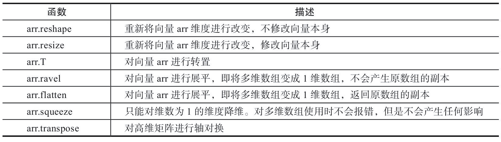
1.4.1 changing array shape
Modifying the shape of a specified array is one of the most common operations in Numpy. There are many methods.
-
reshape
import numpy as np

arr=np.arange(10)
print(arr)

# Transform the vector arr dimension into 2 rows and 5 columns
print(arr.reshape(2, 5))

# When specifying dimensions, you can only specify the number of rows or columns, and - 1 can be used for others
print(arr.reshape(5, -1))
print(arr.reshape(-1, 5))
Output:
[0 1 2 3 4 5 6 7 8 9]
[[0 1 2 3 4]
 [5 6 7 8 9]]
[[0 1]
 [2 3]
 [4 5]
 [6 7]
 [8 9]]
[[0 1 2 3 4]
 [5 6 7 8 9]]
In addition, the reshape function does not support specifying the number of rows and columns, so - 1 is necessary. And the specified number of rows or columns must be divisible.
-
resize
import numpy as np

arr=np.arange(10)
print(arr)

# Transform the vector arr dimension into 2 rows and 5 columns
arr.resize(2,5)
print(arr)
Output:
[0 1 2 3 4 5 6 7 8 9]
[[0 1 2 3 4]
 [5 6 7 8 9]]
-
T (vector transpose)
import numpy as np

arr=np.arange(15).reshape(3,5)
print(arr)

# Transpose the vector arr to 5 rows and 3 columns
print(arr.T)
Output:
[[ 0  1  2  3  4]
 [ 5  6  7  8  9]
 [10 11 12 13 14]]
[[ 0  5 10]
 [ 1  6 11]
 [ 2  7 12]
 [ 3  8 13]
 [ 4  9 14]]
-
T ravel (vector flattening)
import numpy as np

arr=np.arange(6).reshape(2,-1)
print(arr)

#Flatten by column priority
print("Flatten by column priority")
print(arr.ravel('F'))

# Flatten by row
print("Flatten by row")
print(arr.ravel())
Output:
[[0 1 2]
 [3 4 5]]
Flatten by column priority
[0 3 1 4 2 5]
Flatten by row
[0 1 2 3 4 5]
-
flatten (matrix is transformed into vector, which often appears between convolution network and full connection layer)
import numpy as np

a =np.floor(10*np.random.random((3,4)))
print(a)
print(a.flatten())
Output:
[[3. 3. 7. 5.]
 [6. 4. 1. 2.]
 [4. 5. 9. 6.]]
[3. 3. 7. 5. 6. 4. 1. 2. 4. 5. 9. 6.]
-
squeeze (mainly used to reduce the dimension and remove the dimension containing 1 in the matrix)
import numpy as np

arr=np.arange(3).reshape(3,1)
print(arr.shape)  #(3,1)

print(arr.squeeze().shape)   #(3,)

arr1=np.arange(6).reshape(3,1,2,1)
print(arr1.shape)   #(3, 1, 2, 1)

print(arr1.squeeze().shape)  #(3,2)
-
Transfer (axis exchange of high-dimensional matrix)
import numpy as np

arr=np.arange(24).reshape(2,3,4)
print(arr.shape) #(2,3,4)

print(arr.transpose().shape)  #(4,3,2)
1.4.2 merging arrays
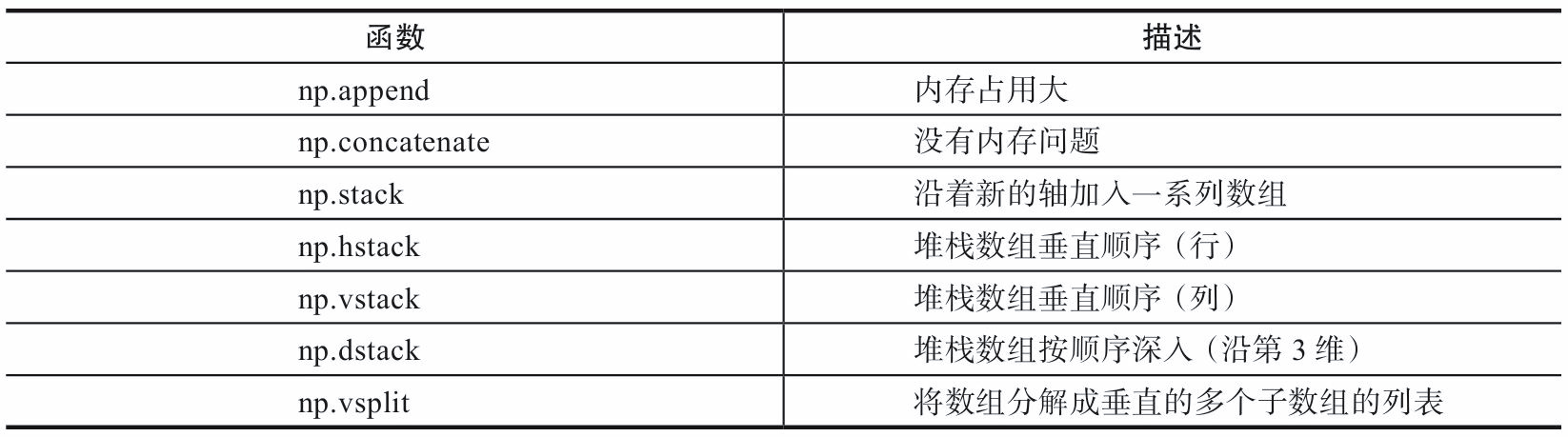
1) append, concatenate, and stack all have an axis parameter to control whether the array is merged by row or column.
2) For append and concatenate, the array to be merged must have the same number of rows or columns (one can be satisfied).
3) stack, hstack, dstack. The arrays to be merged must have the same shape.
- append
import numpy as np

#Merge one-dimensional arrays
a =np.array([1, 2, 3])
b = np.array([4, 5, 6])
c = np.append(a, b)
print(c)  # [1 2 3 4 5 6]
Output:import numpy as np a =np.arange(4).reshape(2, 2) b = np.arange(4).reshape(2, 2) # Merge by row c = np.append(a, b, axis=0) print('Results merged by row') print(c) print('Data dimension after consolidation', c.shape) # Merge by column d = np.append(a, b, axis=1) print('Consolidated results by column') print(d) print('Data dimension after consolidation', d.shape)Results merged by row [[0 1] [2 3] [0 1] [2 3]] Data dimension after consolidation (4, 2) Consolidated results by column [[0 1 0 1] [2 3 2 3]] Data dimension after consolidation (2, 4)
- concatenate (joins an array or matrix along a specified axis)
Output:import numpy as np a =np.array([[1, 2], [3, 4]]) b = np.array([[5, 6]]) c = np.concatenate((a, b), axis=0) print(c) d = np.concatenate((a, b.T), axis=1) print(d)
[[1 2]
 [3 4]
 [5 6]]
[[1 2 5]
 [3 4 6]]
- stack (stacks an array or matrix along a specified axis)
Output:import numpy as np a =np.array([[1, 2], [3, 4]]) b = np.array([[5, 6], [7, 8]]) print(np.stack((a, b), axis=0)) print(np.stack((a, b), axis=1))
[[[1 2]
  [3 4]]

 [[5 6]
  [7 8]]]
[[[1 2]
  [5 6]]

 [[3 4]
  [7 8]]]
1.5 batch processing
In deep learning, batch processing is usually needed because the source data is relatively large. For example, the stochastic gradient method (SGD), which uses batch to calculate the gradient, is a typical application. The calculation of deep learning is generally complex, and the amount of data is generally large. If the whole data is processed at one time, there is a high probability of resource bottleneck. In order to calculate more effectively, the whole data set is generally processed in batches. The other extreme opposite to processing the whole data set is that only one record is processed at a time. This method is also unscientific. Processing one record at a time can not give full play to the parallel processing advantages of GPU and Numpy. Therefore, the mini batch method is often used in practical use. How to split big data into multiple batches? The following steps can be taken:
- Get data set
- Randomly scramble data
- Define batch size
- Batch dataset
Output:import numpy as np #Generate 10000 matrices with shape 2X3 data_train = np.random.randn(10000,2,3) #This is a three-dimensional matrix. The first dimension is the number of samples, and the last two are data shapes print(data_train.shape) #(10000,2,3) #Disrupt these 10000 data np.random.shuffle(data_train) #Define batch size batch_size=1000 #Batch processing for i in range(0,len(data_train),batch_size): x_batch_sum=np.sum(data_train[i:i+batch_size]) print("The first{}batch,Sum of data of this batch:{}".format(i,x_batch_sum))(10000, 2, 3) Batch 0,Sum of data of this batch:-18.08598468837612 Batch 1000,Sum of data of this batch:167.26905751590118 Batch 2000,Sum of data of this batch:-39.48224416996322 Batch 3000,Sum of data of this batch:-74.24661472350503 Batch 4000,Sum of data of this batch:10.274965250772805 Batch 5000,Sum of data of this batch:-56.32505188423596 Batch 6000,Sum of data of this batch:-113.44731706106604 Batch 7000,Sum of data of this batch:-82.65170444631626 Batch 8000,Sum of data of this batch:-51.83454832338842 Batch 9000,Sum of data of this batch:-5.972071452288738
Get data set
2) Randomly scramble data
3) Define batch size
4) Batch dataset
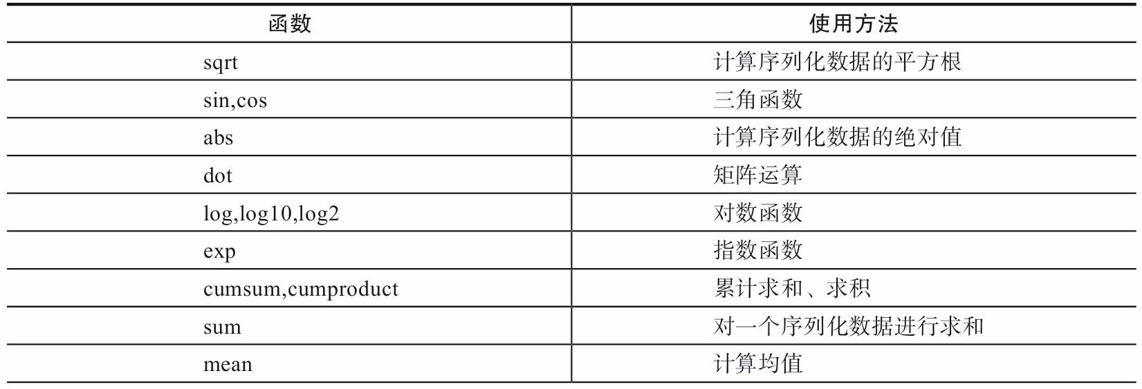
1.6 general functions
Numpy provides two basic objects, the ndarray and ufunc objects. Previously, we introduced ndarray. Here we introduce another object general function (ufunc) of numpy. ufunc is the abbreviation of universal function. It is a function that can operate on each element of an array.
Many ufunc functions are implemented at the C language level, so the calculation speed is very fast. In addition, they are more flexible than the functions in the math module. The input of math module is generally scalar, but the function in Numpy can be vector or matrix, and the use of vector or matrix can avoid circular statements, which is very important in machine learning and deep learning.
- Performance comparison between math and numpy functions
Output:import time import math import numpy as np x = [i * 0.001 for i in np.arange(1000000)] start = time.clock() for i, t in enumerate(x): x[i] = math.sin(t) print ("math.sin:", time.clock() - start ) x = [i * 0.001 for i in np.arange(1000000)] x = np.array(x) start = time.clock() np.sin(x) print ("numpy.sin:", time.clock() - start )
It can be seen that numpy operation is significantly faster than math.math.sin: 0.3137710000000027 numpy.sin: 0.019892999999999716
- Comparison of loop and vector operations
Make full use of the Built-in Function in Python's Numpy library to realize the vectorization of calculation, which can greatly improve the running speed. SIMD instructions are used in the built-in functions in the Numpy library. The vectorization used below is much faster than using loops. If GPU is used, its performance will be more powerful, but Numpy does not support GPU.
Output:import time import numpy as np x1 = np.random.rand(1000000) x2 = np.random.rand(1000000) # Calculating vector dot products using loops tic = time.process_time() dot = 0 for i in range(len(x1)): dot+= x1[i]*x2[i] toc = time.process_time() print ("dot = " + str(dot) + "\n for loop----- Computation time = " + str(1000*(toc - tic)) + "ms") ##Using numpy function to find point product tic = time.process_time() dot = 0 dot = np.dot(x1,x2) toc = time.process_time() print ("dot = " + str(dot) + "\n verctor version---- Computation time = " + str(1000*(toc - tic))+"ms")
It can be seen that the vector operation is efficient, so the vectorization matrix is generally used in the deep learning algorithm.dot = 249746.44050395774 for loop----- Computation time = 630.7314439999984ms dot = 249746.44050396432 verctor version---- Computation time = 2.075084999997756ms
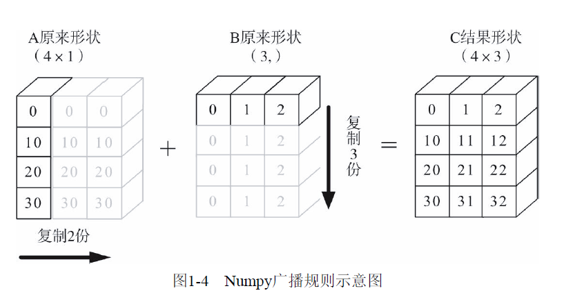
1.7 broadcasting mechanism
Numpy's Universal functions requires that the input array shapes are consistent. When the array shapes are not equal, the broadcast mechanism will be used. However, to adjust the array so that the shape is the same, certain rules need to be met, otherwise an error will occur.
- Let all input arrays align with the array with the longest shape, and the insufficient part is supplemented by adding 1 in front
- The shape of the output array is the maximum value on each axis of the input array shape
- If the length of an axis of the input array and the corresponding axis of the output array are the same, or the length of an axis is 1, this array can be used for calculation, otherwise an error will occur;
- When the length of an axis of the input array is 1, the first set of values on this axis are used (or copied) when operating along this axis.
Output:import numpy as np A = np.arange(0, 40,10).reshape(4, 1) B = np.arange(0, 3) print("A Shape of matrix:{},B Shape of matrix:{}".format(A.shape,B.shape)) C=A+B print("C Shape of matrix:{}".format(C.shape)) print(C)A Shape of matrix:(4, 1),B Shape of matrix:(3,) C Shape of matrix:(4, 3) [[ 0 1 2] [10 11 12] [20 21 22] [30 31 32]]
1.8 summary
The above are common operations of Numpy module, especially matrix operations. For more information, see Numpy official website