explain

The scene is entity recognition. The original version is one by one prediction, which is too inefficient. Here it is changed to parallel prediction.

content

1 processing flow

For each document (from a sentence to a large article), we need to cut sentences first. The goal is to generate short sentences (SS), which will be the input parameter of model processing.

It is agreed that each document is listed in DICTIONARY [{'doc_id':xxx, 'content':xxx},...] Input in a unified way and convert it into DF before processing. If it is tabular, it will be directly converted to df0

doc_id	content
xxx	xxxx

Handle.

First, according to doc_id, and each content is divided into several short sentences df1

doc_id	ss	ss_hash
xxx	xxx	xxx

df1 is temporarily stored, which mainly needs doc_id and ss_hash.

Then df1 is calculated according to ss_hash de duplication, leaving only ss_hash and ss fields to form a new df2

Then df2 is sent into the model. The model circulates according to the length of SS, and processes ss of a certain length each time, and finally forms df3

ss_hash	result
xxx	xxx

Finally, the result of df3 is formed into a dictionary and matched to df2 (according to ss_hash), which is called df4. Will df4 follow doc_id summary and summation get the final result.

doc_id	result
xxx	xxx

The key of parallelization lies in the short sentences with the same length as batch processing.

Note: after sorting out this part, it can also be put into the rule set template, which can be called directly next time.

2 specific process

2.1 Guide Package

import FuncDict as fd
import pandas as pd
cur_func_dict = fd.FuncDict1('parallel_electra', pack_fpath='./funcs/',lmongo=fd.func_lmongo)
import funcs as fs
cur_func_dict.fs = fs
from IPython.display import HTML
import time
import tqdm

2.2 reading data

• There are 1000 pkl files under the folder

the_path = './test_0_1000/manual_data/'
# Get the first n file names - read them in manually this time
cur_batch_flist = fs.get_batch_file(the_path,'query_result_', 2000)
cur_batch_flist1 = [x.replace('.pkl','') for x in cur_batch_flist]
data_list = fs.get_batch_pkl(cur_batch_flist1, the_path, fs)
df_list = []
for the_data in data_list:
    tem_df = pd.DataFrame(list(the_data), columns = ['id','content_a','content_b'])
    df_list.append(tem_df)
df0 = pd.concat(df_list, ignore_index=True)

Among them, df0 is the original data frame to be processed, which should have only one content, but this manual processing is an exception, which is ignored for the time being. Then rename it and run it twice. About 570000 pieces of data were processed this time.

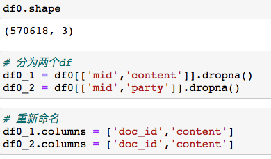
Because there are two calculations, keep one copy of the original data (merge after all calculations)

2.3 split short sentences

# Process first calculation
cur_df0 =  df0_1
the_df = cur_df0.copy()

# Parameter setting
# Think the company name should be no less than 4 words (the person name may be 2)
keep_min_len = 2
keep_max_len = 100
# A short sentence processed in parallel, depending on the video memory
batch_size =4000
target='company'


start = time.time()
# Cut the text
the_df['content_list'] = the_df['content'].apply(fs.txt_etl)
end = time.time()
print('takes %.2f' %(end-start))
---
takes 3.80

Use about 4 seconds to segment the original long string into short sentences

2.4 integrate wide tables into long tables, which is the slowest step

doc_id_list = []
ss_list = []
start = time.time()
for i in range(len(the_df)):
    the_dict = dict(the_df.iloc[i])
    # Missing is not allowed
    the_doc_id = the_dict['doc_id']
    content_list = the_dict['content_list']
    content_list1 = [x for x in content_list if len(x)>=keep_min_len and len(x) < keep_max_len]
    tem_doc_id_list = [the_doc_id] * len(content_list1)
    doc_id_list += tem_doc_id_list
    ss_list  += content_list1

end = time.time()
print('takes %.2f' %(end-start))
---
takes 53.23

2.5 processing short sentences

Because the company name / person name is to be analyzed, the short sentences should be further cleaned

start = time.time()
df1 = pd.DataFrame()
df1['doc_id'] = doc_id_list
df1['ss'] = ss_list
# Screen the short sentences again
df1['ss'] = df1['ss'].apply(fs.extract_str_like_company_human)
df1['ss_hash'] = df1['ss'].apply(fs.md5_trans)
end = time.time()
print('takes %.2f' %(end-start))
---
takes 13.13

2.6 further screening short sentences

The company name is calculated this time, so it can be further screened

start = time.time()
# There are characteristic words for the company
sel = (df1['ss'].apply(len) >3) & (df1['ss'].apply(fs.str_contains_words))
end = time.time()
print('takes %.2f' %(end-start))
---
takes 17.78

Last hold data

# Finally, there may be documents and short sentences with data
df2 = df1[sel][['doc_id', 'ss_hash']].copy()
# Keep df2 for the final result
df2.shape
---
(1244248, 2)

df2 = df2.drop_duplicates()
df2.shape
(1243764, 2)

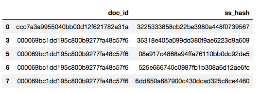
2.7 df to be processed in model generation

The repeated ss can be removed, and there is no need for repeated processing

# According to ss_hash de duplication
df3 = df1[sel][['ss_hash','ss']].drop_duplicates(['ss_hash']).copy()

# Finally, cycle according to the length
df3['ss_len']= df3['ss'].apply(len)

# Store dictionary with length as key value
ss_res_dict = {}
for i in range(keep_min_len,keep_max_len):
    ss_res_dict[i] = df3[df3['ss_len']==i]['ss']


# Each item in the list is batch processed by the model
all_length_ss_list = []
for k in list(ss_res_dict.keys()):
    cur_ss = ss_res_dict[k]
    # Considering the video memory / memory, the data will be segmented once more (if it is too long, it will be cut into n segments)
    cur_ss_list = fs.split_series_by_interval(cur_ss, batch_size)
    all_length_ss_list += cur_ss_list

2.8 model parameter setting

These are the same settings as during training

# Model initial settings
path_name = './'
model_checkpoint = path_name + 'model/model_v0/'
label_list = ['O', 'B-PER', 'I-PER', 'B-ORG', 'I-ORG', 'B-LOC', 'I-LOC', 'B-T', 'I-T']
max_len = 200
import torch
import transformers
from transformers import AutoTokenizer, AutoModelForTokenClassification

# Setting up the device for GPU usage
from torch import cuda
device = 'cuda' if cuda.is_available() else 'cpu'
print('device available', device)
tokenizer = AutoTokenizer.from_pretrained(model_checkpoint)
assert isinstance(tokenizer, transformers.PreTrainedTokenizerFast)
# Preload (device=cpu)
model = AutoModelForTokenClassification.from_pretrained(model_checkpoint, num_labels=len(label_list))
from functools import partial 
tencoder = partial(tokenizer.encode,truncation=True, max_length=max_len, is_split_into_words=True, return_tensors="pt")

---
device available cuda

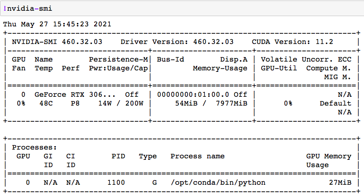
2.9 cyclic treatment

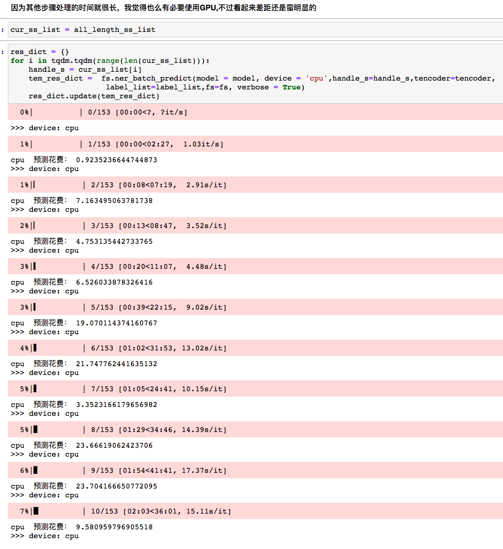
Call the parallel processing of the model once for each list. Here you can see the gap between CPU and GPU

cur_ss_list = all_length_ss_list
res_dict = {}
for i in tqdm.tqdm(range(len(cur_ss_list))):
    handle_s = cur_ss_list[i]
    tem_res_dict =  fs.ner_batch_predict(model = model, device = 'cuda',handle_s=handle_s,tencoder=tencoder,
                     label_list=label_list,fs=fs, verbose = True)
    res_dict.update(tem_res_dict)

2.9.1 CPU processing

CPU processing time varies with the size of the object.

2.9.2 GPU processing

If the video memory does not explode, the processing time of GPU is almost constant.

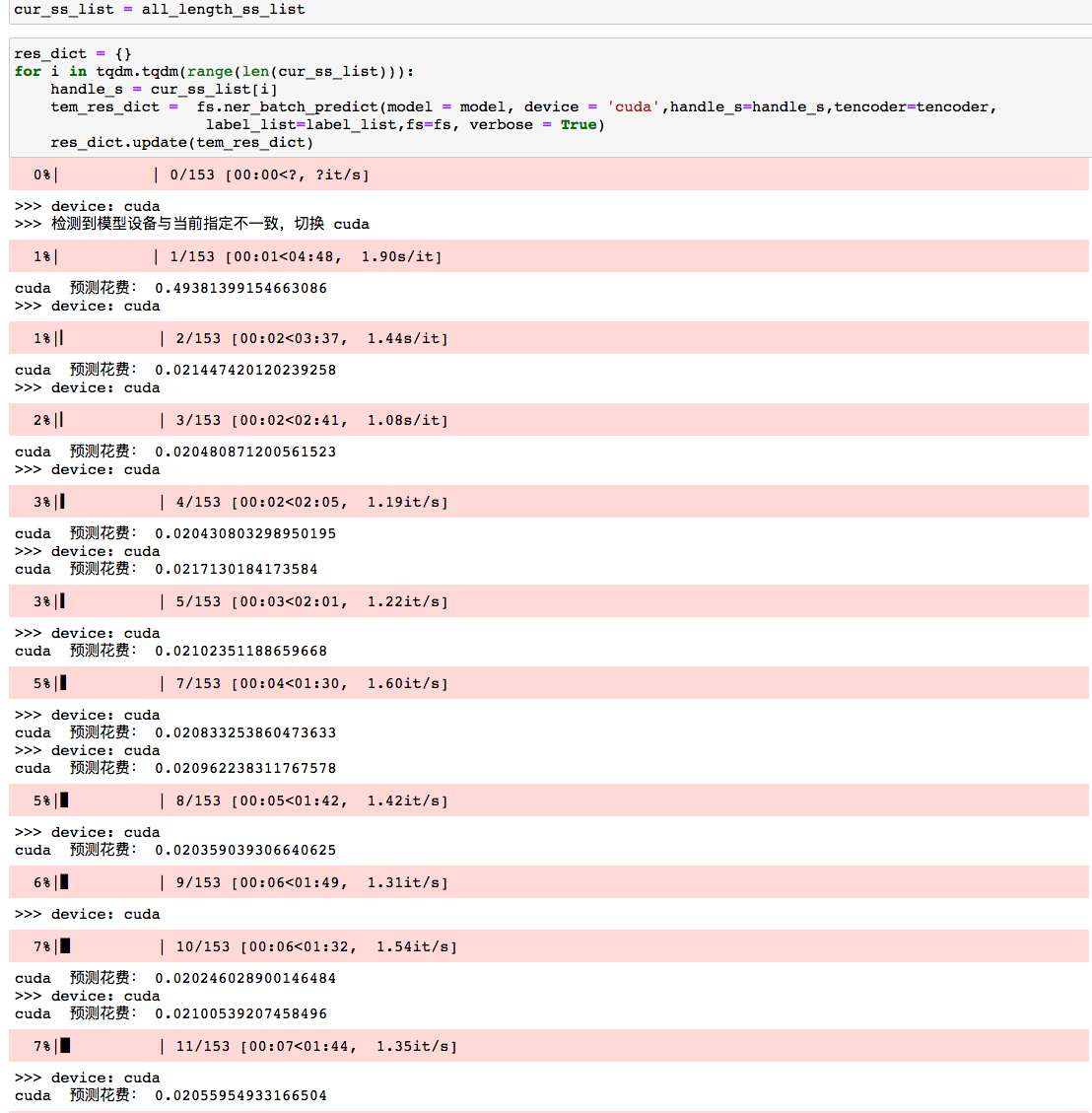
After evaluation, it is estimated that the CPU takes 1500 seconds (ten seconds on average) and the GPU takes 3 seconds (0.02 on average) to process the 150 list elements. In the original single shot model, each document needs to be processed for 0.3 seconds. In the previous data processing overhead, we think there are 200 seconds, and the data is estimated as 500000 pieces.

pattern	Average time per document
single shot	0.3s
Concurrent CPU	0.0034s
Concurrent GPU	0.0004s

The use of graphics card makes the model prediction not a bottleneck in the process.

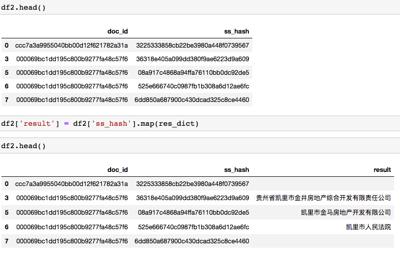
2.10 merge the results into df2 and output them as documents

2.10.1 press SS first_ Hash matches the prediction results of the model

2.10.2 screening by length

I wrote an Interval judgment function myself, so I don't need to install the Interval package.

# Set retention interval
keep_min_len = 4
keep_max_len = 100
# Default left closed right open
keep_interval = fs.set_interval_judge(xleft = keep_min_len, xright = keep_max_len, fs = fs)

df2.shape
---
(1243764, 3)

df4 = df2.dropna()
# str.strip() is to delete the spaces at the beginning and end of the string, as well as the spaces \ n \t at the beginning and end of the string.
sel4 = df4['result'].apply(lambda x: str(x).strip()).apply(len).apply(keep_interval)
sel4.sum()
---
698142

df_res = df4[sel4].copy()

2.10.3 combined output

df_res['result'] = df_res['result'] +','

start = time.time()
df_res1 = df_res.groupby(['doc_id'])['result'].sum().reset_index()
end = time.time()
print('takes %.2f' %(end-start))
---
takes 42.27

3 Summary

• 1 parallelization is 100 times faster than single processing
• 2. Computing with graphics card is at least 20 times faster than CPU
• 3 the next step is to do some standardization to package
• 4. The mode will change when the interface is called. The first request will receive a receipt, but it may take several minutes to get the result. (handling 100000 pieces at a time is appropriate)
• 5 if there is a large amount of requests, you can save the results of ss in the database as a dictionary. Most of the time, it is disassembled into short sentences and use ss_hash query is good. There is no need to calculate repeatedly.