1. Color image processing

1.1 image reading

Use the python PIL library to read the Image. This method returns an Image object. The Image object stores the format (jpeg,jpg,ppm, etc.), size and color mode (RGB) of the Image. It contains a show() method to display the Image:

# Import PIL Library
from PIL import Image
# Use the Image class to read images
img = Image.open("Image-Progcess/image.png")
# View image information
print(img.format,img.size,img.mode)
# Display image
img.show()

Reading an image does not require its format.

1.2 write image

To write an Image file in different formats using an Image object, you need to specify its format:

# Write image
# The system library is introduced to provide the method of obtaining the directory
# Import PIL Library
from PIL import Image
import os,sys
​
# The Image object uses the save method to store the Image file
# Convert file to JPEG
# sys.argv[1:] is the parameter [args] when calling the python module using python file.py [args]
for infile in sys.argv[1:]:
    f,e = os.path.splitext(infile)
    outfile = f + ".png"
    print(outfile)
    if infile != outfile:
        try:
            img = Image.open("image.png")
            print(img.size)
            with Image.open(outfile) as im:
                print(im.size)
                im.save(f+'.jpg')
                im.save(f+'.ppm')
                im.save(f+'.bmp')
        except OSError as e:
            print('cannot convert',str(e))

1.3 (bitmap) introduction to BMP image format

BMP format, also known as Bitmap, is an image file format widely used in Windows system. Because it can save the data of image pixel domain without any transformation, it has become an important source for us to obtain RAW data.

The data of BMP file is divided into four parts according to the order of file header:

• bmp file header: provides file format, size and other information
• Bitmap header: provides the size of image data, number of bit planes, compression mode, color index and other information.
• Palette (optional): this section is optional, and the color is represented by index.

1.3 bits of bitmap (BMP) (32 bits, 16 bits)

Bitmaps are represented by an array of bits. 32 bits and 16 bits represent the color quality, that is, how many bits are used for each pixel (1, 4, 8, 15, 24, 32 or 64). This number is specified in the file header.

1.4 color number of bitmap (256 colors, 16 colors, monochrome)

The color number of bitmap is determined by the palette. Only 4 and 8-bit images use palette data. 16, 24 and 32-bit images do not need palette data. The palette only needs 256 items at most (index 0 - 255). The size of the palette depends on the color mode used: 2-color images are 8 bytes; 16 color image bits 64 bytes; 256 color images are 1024 bytes.

1.5 image format (BMP, JPG, GIF, PNG)

2. Machine vision

2.1 introduction to singular value decomposition (SVD)

Singular value decomposition is one of the matrix decomposition methods. It decomposes the matrix into three sub matrices, namely U, S and V, where U is the left eigenvector, S is the diagonal matrix of singular value, and V is called the right eigenvector.

The image SVD matrix is reconstructed using numpy's linalg.svd() method.

linalg.svd(Matrix, full_matrices=True，compute_uv=True，hermitian=False)

Parameters:

1. Matrix: real or complex matrix with size > 2.
2. full_matrices: if True, the size of u and v matrices is mxn; if False, the shape of u and v matrices is mxk, where k is only a non-zero value.
3. compute_uv: use Boolean values to calculate u and v matrices and s matrix.
4. Hermitian: by default, if the matrix contains real values, it is assumed that the matrix is Hermitian, which is internally used to effectively calculate singular values.

2.2 singular value decomposition (SVD) is used to reduce the dimension of the picture

2.2.1 read image

Use the linalg.svd() method to decompose the matrix to see how many linearly independent feature vectors the image has.

# Import module
import requests
import cv2
import numpy as np
import matplotlib.pyplot as plt
​
# Assign and open images
url = 'https://media.geeksforgeeks.org/wp-content/cdn-uploads/20210401173418/Webp-compressed.jpg'
response = requests.get(url, stream=True)
​
with open('image.png', 'wb') as f:
    f.write(response.content)
​
img = cv2.imread('image.png')
​
# Convert images to grayscale to speed up
# calculation.
gray_image = cv2.cvtColor(img, cv2.COLOR_BGR2GRAY)
​
# Calculate SVD
u, s, v = np.linalg.svd(gray_image, full_matrices=False)
​
# Check the shape of the matrix
print(f'u.shape:{u.shape},s.shape:{s.shape},v.shape:{v.shape}')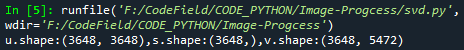

The output shape shows that the image has 3648 linearly independent feature vectors.

2.2.2 viewing the variance of images used in singular vectors

# Import module
import seaborn as sns
 
var_explained = np.round(s**2/np.sum(s**2), decimals=6)
 
# Variance interpretation top singular vector
print(f'variance Explained by Top 20 singular values:\n{var_explained[0:20]}')
 
sns.barplot(x=list(range(1, 21)),
            y=var_explained[0:20], color="dodgerblue")
 
plt.title('Variance Explained Graph')
plt.xlabel('Singular Vector', fontsize=16)
plt.ylabel('Variance Explained', fontsize=16)
plt.tight_layout()
plt.show()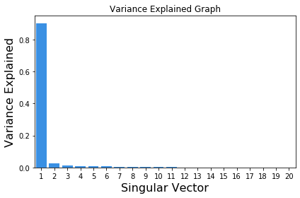

The variance interpretation diagram above shows that about 99.77% of the information is explained by the first eigenvector and its corresponding eigenvalue itself.

2.2.3 only the first few feature vectors are used to reconstruct the image

Reorganize the image using a different number of singular values:

# Draw images with different numbers of singular values
comps = [3648, 1, 5, 10, 15, 20]
plt.figure(figsize=(12, 6))
 
for i in range(len(comps)):
    low_rank = u[:, :comps[i]] @ np.diag(s[:comps[i]]) @ v[:comps[i], :]
     
    if(i == 0):
        plt.subplot(2, 3, i+1),
        plt.imshow(low_rank, cmap='gray'),
        plt.title(f'Actual Image with n_components = {comps[i]}')
     
    else:
        plt.subplot(2, 3, i+1),
        plt.imshow(low_rank, cmap='gray'),
        plt.title(f'n_components = {comps[i]}')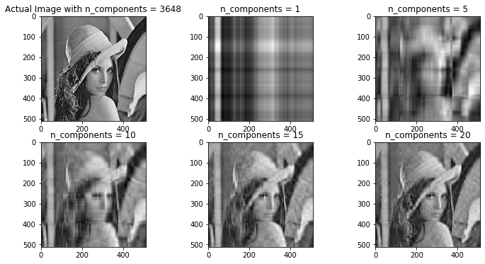

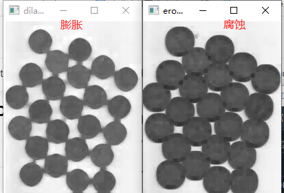
2.3 image opening and closing operation (corrosion expansion)

2.3.1 corrosion

The basic idea of erosion is like soil erosion, which erodes the boundary of the foreground object (always try to keep the foreground white). So what does it do? The kernel slides in the image (as in 2D convolution). Only when all pixels under the kernel are 1, the pixel (1 or 0) in the original image will be regarded as 1, otherwise it will be eroded (make it zero).

The corrosion operation is to replace the value of the central pixel covered by the structural element with the minimum value:

import cv2
import numpy as np
​
img = cv2.imread('j.png',0)
kernel = np.ones((5,5),np.uint8)
erosion = cv2.erode(img,kernel,iterations = 1)

2.3.2 expansion

The expansion operation is to replace the value of the central pixel covered by the structural element with the maximum value:

dilation = cv2.dilate(img,kernel,iterations = 1)

2.3.3 Hough circles

HoughCircles() function only accepts single channel images. Before using images, use cv2.cvtColor() function to obtain gray-scale images:

# Gray image
gray = cv2.cvtColor(img,cv2.COLOR_BGR2GRAY)

Circle drawing function using Hough circle Transformation:

# Draw a circle
def drawCircle(image):
    # Hoff circle transformation
    circles = cv2.HoughCircles(
    image,
    cv2.HOUGH_GRADIENT,
    1,
    20,
    param1=50,
    param2=30,
    minRadius=0,
    maxRadius=0
    )
    
    # Make sure at least some circles are found
    output = image.copy()
    if circles is not None:
        # Converts the (x, y) coordinates and radius of a circle to an integer
        circles = np.round(circles[0, :]).astype("int")
        # Circular (x, y) coordinates and radius of circle
        for (x, y, r) in circles:
            # Draw a circle in the output image, and then draw a rectangle
            # Corresponding center
            cv2.circle(output, (x, y), r, (0, 255, 0), 4)
        # Display output image
        cv2.imshow("output", np.hstack([image, output]))
        cv2.waitKey(0)

1) Using fuzzy gray image and Hough circle transform

img = cv2.imread('Image-Progcess/image1.png')
# Gray image
gray = cv2.cvtColor(img,cv2.COLOR_BGR2GRAY)
# Fuzzy gray image 
blurred = cv2.medianBlur(gray,5)
# Draw a circle
drawCircle(blurred)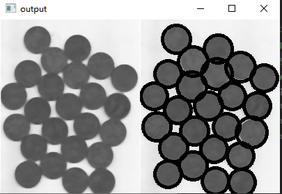

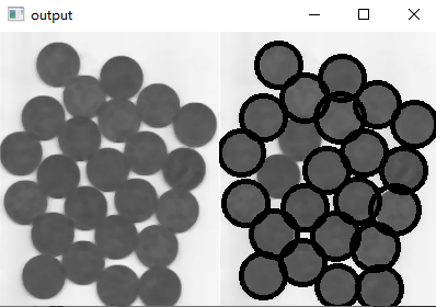
2) Using corrosion operation and Hough circle transformation

erosion = cv2.erode(img,kernel,iterations = 1)

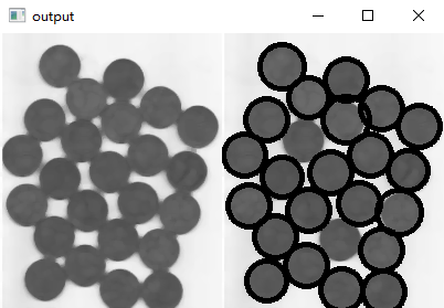
3) Use expansion operation

dilation = cv2.dilate(img,kernel,iterations = 1)

2.4 image gradient, opening and closing, contour operation

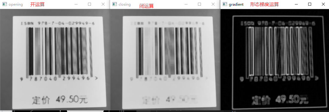
2.4.1 opening and closing operation, morphological gradient

The disconnection operation is to corrode the image first, and then expand the image. The disconnection operation can disconnect the connectivity of two objects. Realize object separation.

The closed operation uses structural elements to expand the image first and then corrode it, which is just the opposite order of the open operation, but the closed operation is definitely not the reverse result of the open operation.

The gradient operation of morphology is the difference between image expansion and corrosion results:

# Open operation
opening = cv2.morphologyEx(img, cv2.MORPH_OPEN, kernel)
# Closed operation
closing = cv2.morphologyEx(img, cv2.MORPH_CLOSE, kernel)
#Morphological gradient
gradient = cv2.morphologyEx(img, cv2.MORPH_GRADIENT, kernel)

2.4.2 object contour detection using edges

In order to detect circles or any other geometry, we first need to detect the edges of objects existing in the image.

The edges in the image are points with sharp color changes. For example, the edge of a red ball on a white background is a circle. In order to recognize the edge of an image, a common method is to calculate the image gradient.

Find the outline of the image:

cnts = cv2.findContours(closed.copy(), cv2.RETR_EXTERNAL, cv2.CHAIN_APPROX_SIMPLE)

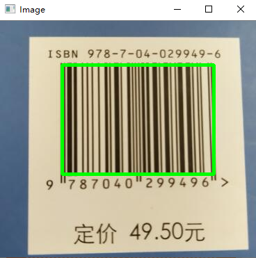
2.4.3 bar code detection

# Import required libraries
import numpy as np
import imutils
import cv2
# Convert to grayscale image
image = cv2.imread('Image-Progcess/tiaoxingma2.jpg')
gray = cv2.cvtColor(image, cv2.COLOR_BGR2GRAY)
# Edge detection method using Scharr operator
ddepth = cv2.CV_32F if imutils.is_cv2() else cv2.CV_32F
gradX = cv2.Sobel(gray, ddepth=ddepth, dx=1, dy=0, ksize=-1)
gradY = cv2.Sobel(gray, ddepth=ddepth, dx=0, dy=1, ksize=-1)
gradient = cv2.subtract(gradX,gradY)
gradient = cv2.convertScaleAbs(gradient)
#Noise removal
## Fuzzy and thresholding processing
blurred = cv2.blur(gradient,(9, 9))
(_, thresh) = cv2.threshold(blurred, 231, 255, cv2.THRESH_BINARY)
## Morphological processing
kernel = cv2.getStructuringElement(cv2.MORPH_RECT, (21, 7))
closed = cv2.morphologyEx(thresh, cv2.MORPH_CLOSE, kernel)
closed = cv2.erode(closed, None, iterations=4)
closed = cv2.dilate(closed, None, iterations=4)
# Determine the detection contour and draw the detection box
cnts = cv2.findContours(closed.copy(), cv2.RETR_EXTERNAL, cv2.CHAIN_APPROX_SIMPLE)
cnts = imutils.grab_contours(cnts)
c = sorted(cnts, key=cv2.contourArea, reverse=True)[0]
 
rect = cv2.minAreaRect(c)
box = cv2.boxPoints(rect) if imutils.is_cv2() else cv2.boxPoints(rect)
box = np.int0(box)
 
cv2.drawContours(image, [box], -1, (0, 255, 0), 3)
cv2.imshow("Image", image)
cv2.waitKey(0)
cv2.destroyAllWindows()

3. Reference

python+OpenCV detect barcode

Image morphological operation in OpenCV