[python drawing] common settings of Matplotlib

Symbol	Chinese description	English description
'.'	Dot	point marker
','	Pixel point	pixel marker
'o'	circle	circle marker
'v'	Downward triangle	triangle_down marker
'^'	Upward triangle	triangle_up marker
'<'	Left triangle	triangle_left marker
'>'	Right triangle	triangle_right marker
'1'	Downward Y-shape	tri_down marker
'2'	Up Y	tri_up marker
'3'	Left Y	tri_left marker
'4'	Right Wye	tri_right marker
's'	square	square marker
'p'	pentagon	pentagon marker
'*'	star	star marker
'h'	Hexagon 1	hexagon1 marker
'H'	Hexagon 2	hexagon2 marker
'+'	plus	plus marker
'x'	Cross sign	x marker
'D'	Diamond shape	diamond marker
'd'	Diamond shape (small)	thin_diamond marker
'\|'	Vertical line	vline marker
'_'	Horizontal line	hline marker

Line Styles supported by matplotlib

Symbol	Chinese description	English description
'-'	Solid line	solid line style
'--'	Dotted line	dashed line style
'-.'	Dotted line	dash-dot line style
':'	Point line	dotted line style

Color abbreviations supported by matplotlib (Colors)

Symbol	Chinese description	English description
'b'	blue	blue
'g'	green	green
'r'	red	red
'c'	young	cyan
'm'	purple	magenta
'y'	yellow	yellow
'k'	black	black
'w'	white	white

Comparison of Chinese and English names of Windows fonts

Chinese name	English name
Blackbody	SimHei
Microsoft YaHei	Microsoft YaHei
Microsoft JhengHei	Microsoft JhengHei
NSimSun	NSimSun
New fine bright body	PMingLiU
Fine bright body	MingLiU
DFKai-SB	DFKai-SB
Imitation Song Dynasty	FangSong
Regular script	KaiTi
Imitation Song Dynasty_ GB2312	FangSong_GB2312
Regular script_ GB2312	KaiTi_GB2312

Object oriented drawing

matplotlib is a set of object-oriented drawing library. All parts in the drawing are python objects.
pyplot is a set of fast drawing API provided by matplotlib, which imitates MATLAB. It is not the ontology of matplotlib.
Although pyplot is simple and fast to use, it hides a lot of details and cannot use some advanced functions.
The pyplot module stores information such as the current chart and current sub chart, which can be obtained by gcf() and gca() respectively:

plt.gcf(): "Get current figure" to get the current chart (Figure object)

plt.gca(): "Get current figure" to get the current subgraph (Axes object)

All kinds of drawing functions in pyplot are actually internally calling gca to get the current Axes object, and then calling Axes to complete the drawing.

import matplotlib.pyplot as plt
# Get the current Figure and Axes objects
plt.figure(figsize=(4,3))
fig = plt.gcf()
axes = plt.gca()
print(fig)
print(axes)

Configure the properties of the object

Each part of the chart drawn by matplotlib corresponds to an object. There are two ways to set the properties of these objects:

set through object_* () method setting.

Set through the setp() method of pyplot.

There are also two ways to view the properties of an object:

get through object_* () method view.

View through the getp() method of pyplot.

import matplotlib.pyplot as plt
import numpy as np
# Get the current Figure and Axes objects
plt.figure(figsize=(4,3))
fig = plt.gcf() ; axes = plt.gca()
print(fig); print(axes)
x = np.arange(0, 5, 0.1)
# Call the plot.plot function to return a list of Line2D objects
lines = plt.plot(x, 0.05*x*x); print(lines)
# Call the set series method of the Line2D object to set the property value
# With set_alpha sets the alpha channel, that is, transparency
lines[0].set_alpha(0.5) ; plt.show()
# The plot.plot function can accept an indefinite number of position parameters. These position parameters are paired to generate multiple curves.
lines = plt.plot(x, np.sin(x), x, np.cos(x), x, np.tanh(x))
plt.show()
# Use the plt.setp function to configure the properties of multiple objects at the same time. Here, set the color and lineweight of all curves in the lines list.
plt.setp(lines, color='r', linewidth=4.0);plt.show()
# Use the getp method to view all properties
f = plt.gcf(); plt.getp(f)

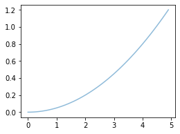
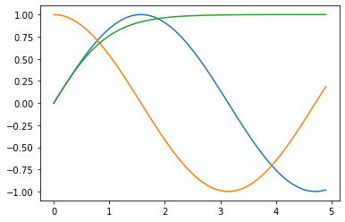
import numpy as np
import matplotlib.pyplot as plt
# Get the current Figure and Axes objects
plt.figure(figsize=(4,3))
fig = plt.gcf() ; axes = plt.gca()
print(fig); print(axes)
x = np.arange(0, 5, 0.1)
# Call the plot.plot function to return a list of Line2D objects
lines = plt.plot(x, 0.05*x*x); print(lines)
# Call the set series method of the Line2D object to set the property value
# With set_alpha sets the alpha channel, that is, transparency
lines[0].set_alpha(0.5) ; plt.show()
# The plot.plot function can accept an indefinite number of position parameters. These position parameters are paired to generate multiple curves.
lines = plt.plot(x, np.sin(x), x, np.cos(x), x, np.tanh(x))
plt.show()
# Use the plt.setp function to configure the properties of multiple objects at the same time. Here, set the color and lineweight of all curves in the lines list.
plt.setp(lines, color='r', linewidth=4.0);plt.show()
# Use the getp method to view all properties
f = plt.gcf(); plt.getp(f)
# View a property
print(plt.getp(lines[0],"color"))
# get using object_* () method
print(lines[0].get_linewidth())
# The axes attribute of the Figure object is a list that stores all axes objects in the Figure.
# The following code checks the axes attribute of the current Figure, that is, the current axes object obtained by gca.
print(plt.getp(f, 'axes'))
print(len(plt.getp(f, 'axes')))
print(plt.getp(f, 'axes')[0] is plt.gca())
# Use plt.getp() to continue to obtain the properties of the AxesSubplot object. For example, its lines property is the list of Line2D objects in the subgraph.
# In this way, you can view the attribute values of objects and the relationship between objects.
all_lines = plt.getp(plt.gca(), "lines");print(all_lines)
plt.close() # Close current chart

Draw multiple subgraphs

In matplotlib, a Figure object can include multiple Axes objects (that is, subgraphs), and one axis represents a drawing area. The simplest way to draw multiple subgraphs is to use the subplot function of pyplot.
subplot(numRows, numCols, plotNum) accepts three parameters:

numRows: number of subgraph rows

numCols: number of subgraph columns

plotNum: the number of subgraphs (numbered from left to right and from top to bottom)

import matplotlib.pyplot as plt
# Create 3 rows and 2 columns, totaling 6 subgraphs.
# subplot(323) is equivalent to subplot(3,2,3).
# The number of subgraphs starts from 1, not 0.
fig = plt.figure(figsize=(4,3))
for idx,color in enumerate('rgbcyk'):
    plt.subplot(321+idx, facecolor=color)
plt.show()
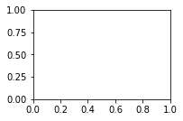
# If the newly created subgraph overlaps with the previously created subgraph, the previous subgraph will be deleted
plt.subplot(221)
plt.show()
plt.close()
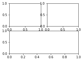
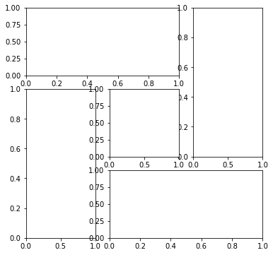
# Multiple subgraphs with different heights or widths can also be spliced with each other
fig = plt.figure(figsize=(4,3))
plt.subplot(221) # First row left
plt.subplot(222) # First row right
plt.subplot(212) # The second line is the whole line
plt.show()
plt.close()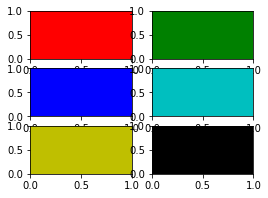

Artist object

Simple type Artist objects are standard drawing components, such as Line2D, Rectangle, Text, AxesImage, etc

The Artist object of container type contains multiple Artist objects to organize them into a whole, such as Axis, Axes and Figure objects

Process of drawing with Artist object

Create Figure object
Create one or more Axes objects for the Figure object
Call the methods of the Axes object to create various simple Artist objects

import matplotlib.pyplot as plt
fig = plt.figure()
# The list is used to describe the location of the picture and the size of the picture
ax = fig.add_axes([0.15, 0.1, 0.7, 0.3])
ax.set_xlabel('time')
line = ax.plot([1, 2, 3], [1, 2, 1])[0]
# The lines attribute of ax is a list of all curves
print(line is ax.lines[0])
# Through get_* Get the corresponding properties
print(ax.get_xaxis().get_label().get_text())
plt.show()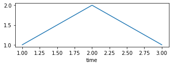

Set Artist properties

get_* And set_* Function to read and write fig.set_alpha(0.5*fig.get_alpha())

Artist property	effect
alpha	Transparency, values between 0 and 1, 0 is fully transparent and 1 is fully opaque
animated	Boolean value used when drawing animation effects
axes	The Axes object where this Artist object is located may be None
clip_box	Object's crop box
clip_on	Crop
clip_path	Clipped path
contains	A function that determines whether a specified point is on an object
figure	The Figure object in which it is located may be None
label	Text label
picker	Control Artist object selection
transform	Control offset rotation
visible	Visible
zorder	Control drawing order

Some examples

import matplotlib.pyplot as plt
fig = plt.figure()
# Set background color
fig.patch.set_color('g')
# The interface must be updated to be effective
fig.canvas.draw()
plt.show()
# All attributes of the artist object can be obtained through the corresponding get_* () and set_* () read and write
# For example, set the transparency of the following image
line = plt.plot([1, 2, 3, 2, 1], lw=4)[0]
line.set_alpha(0.5)
line.set(alpha=0.5, zorder=1)
# fig.canvas.draw()
# Output all attribute names and corresponding values of the Artist object
print(fig.patch)
plt.show()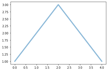

import matplotlib.pyplot as plt
fig = plt.figure()
fig.subplots_adjust(top=0.8)
ax1 = fig.add_subplot(211)
ax1.set_ylabel('volts')
ax1.set_title('a sine wave')
t = np.arange(0.0, 1.0, 0.01)
s = np.sin(2*np.pi*t)
line, = ax1.plot(t, s, color='blue', lw=2)
# Fixing random state for reproducibility
np.random.seed(19680801)
ax2 = fig.add_axes([0.15, 0.1, 0.7, 0.3])
n, bins, patches = ax2.hist(np.random.randn(1000), 50,
    facecolor='yellow', edgecolor='orange')
ax2.set_xlabel('time (s)')
plt.show()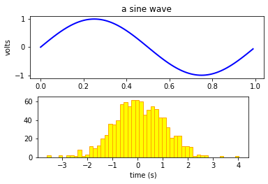

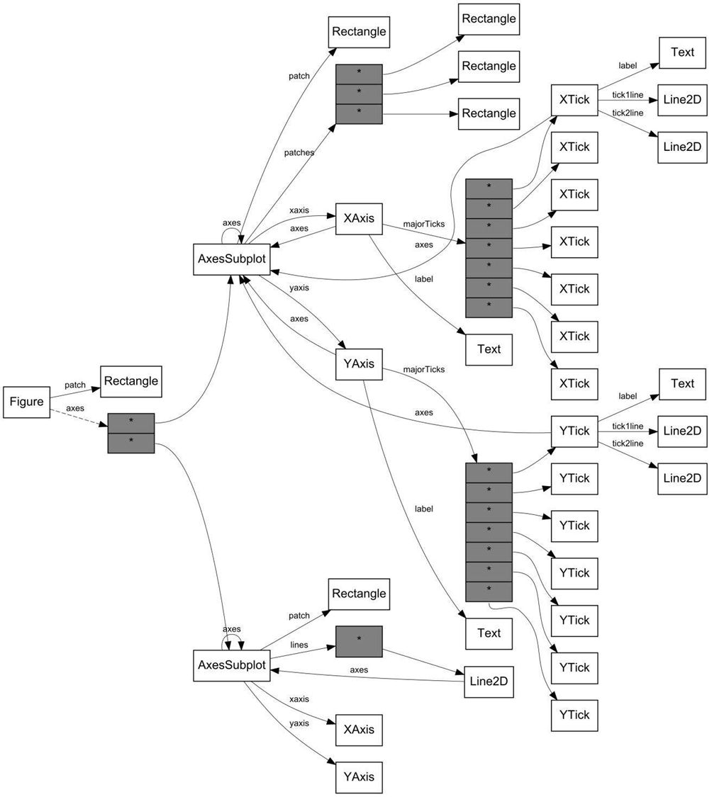
Figure container

The uppermost Artist object is Figure, which contains all the elements that make up the chart

Figure can include multiple Axes (multiple charts). There are three main methods to create them:

axes = fig.add_axes([left, bottom, width, height])
Fig, axes = plt.subplots (number of rows and columns)
axes = fig.add_ Subplot (number of rows, number of columns, sequence number)

Figure attribute	explain
axes	Axis object list
patch	Rectangle object as background
images	FigureImage object list, used to display pictures
legends	Legend object list
lines	Line2D object list
patches	patch object list
texts	A list of Text objects used to display Text

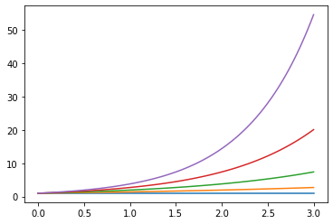
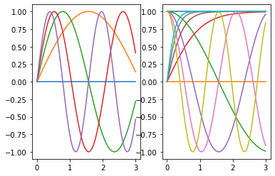
import matplotlib.pyplot as plt
# Let's take a look at an example of flexible switching between multiple figures and multiple Axes.
plt.figure(1) # Create chart 1
plt.figure(2) # Create chart 2
ax1 = plt.subplot(121) # Create subgraph 1 in chart 2
ax2 = plt.subplot(122) # Create subgraph 2 in chart 2
x = np.linspace(0, 3, 100)
for i in range(5):
    plt.figure(1) # Switch to chart 1
    plt.plot(x, np.exp(i*x/3))
    plt.sca(ax1) # Select subgraph 1 of chart 2
    plt.plot(x, np.sin(i*x))
    plt.sca(ax2) # Select subgraph 2 of chart 2
    plt.plot(x, np.cos(i*x))
    ax2.plot(x, np.tanh(i*x)) # You can also plot directly through the plot method of ax2
plt.show()
plt.close() # Two Figure objects are open, so plt.close() is executed twice
plt.close()
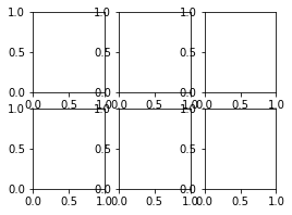
# You can also use the subplots function to generate multiple subgraphs at a time and return an array of Figure objects and Axes objects.
# Note that the difference between subplot and subplots is one s. The former generates subgraphs one by one, and the latter generates subgraphs in batch.
fig, axes = plt.subplots(2, 3, figsize=(4,3))
[a,b,c],[d,e,f] = axes
print(axes.shape)
print(b)
plt.show()
plt.close()

Axes container

Area of the image with data space (marked as internal blue box)
A drawing can contain multiple Axes, and an axis object can contain only one drawing
Axes contains two (or three) Axis objects that are responsible for data restrictions
Each axis has a title (set by set_title()), an x label (set by set_xLabel()), and an x label (set by set_xLabel())_ The y label set set set by ylabel().

Axes property	explain
artists	A list of Artist instances
patch	Rectangle instance for Axes background
collections	A list of Collection instances
images	A list of AxesImage
legends	A list of Legend instances
lines	A list of Line2D instances
patches	A list of Patch instances
texts	A list of Text instances
xaxis	matplotlib.axis.XAxis instance
yaxis	matplotlib.axis.YAxis instance

Helper method of Axes	Created object (Artist)	List of added (Container)
ax.annotate - text annotations	Annotate	ax.texts
ax.bar - bar charts	Rectangle	ax.patches
ax.errorbar - error bar plots	Line2D and Rectangle	ax.lines and ax.patches
ax.fill - shared area	Polygon	ax.patches
ax.hist - histograms	Rectangle	ax.patches
ax.imshow - image data	AxesImage	ax.images
ax.legend - axes legends	Legend	ax.legends
ax.plot - xy plots	Line2D	ax.lines
ax.scatter - scatter charts	PolygonCollection	ax.collections
ax.text - text	Text	ax.texts

The subplot2grid function performs a more complex layout. subplot2grid(shape, loc, rowspan=1, colspan=1, **kwargs)

Shape is the tuple (number of rows and columns) representing the shape of the table
loc is the coordinate tuple (row, column) in the upper left corner of the subgraph
rowspan and colspan are the number of rows and columns occupied by the subgraph, respectively

import matplotlib.pyplot as plt
fig = plt.figure(figsize=(6,6))
ax1 = plt.subplot2grid((3,3),(0,0),colspan=2)
ax2 = plt.subplot2grid((3,3),(0,2),rowspan=2)
ax3 = plt.subplot2grid((3,3),(1,0),rowspan=2)
ax4 = plt.subplot2grid((3,3),(2,1),colspan=2)
ax5 = plt.subplot2grid((3,3),(1,1))
plt.show()
plt.close()

Scale line, scale text, coordinate grid and axis title on coordinate axis, etc

set_major_* set_minor_*

get_major_* get_minor_*

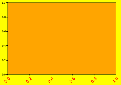
import numpy as np
import matplotlib.pyplot as plt
# plt.figure creates a matplotlib.figure.Figure instance
fig = plt.figure()
rect = fig.patch # a rectangle instance
rect.set_facecolor('yellow')
ax1 = fig.add_axes([0.1, 0.3, 1,1])
rect = ax1.patch
rect.set_facecolor('orange')
for label in ax1.xaxis.get_ticklabels():
    # label is a Text instance
    label.set_color('red')
    label.set_rotation(45)
    label.set_fontsize(16)
for line in ax1.yaxis.get_ticklines():
    # line is a Line2D instance
    line.set_color('green')
    line.set_markersize(5)
    line.set_markeredgewidth(3)
plt.show()

Axis scale setting

matplotlib will automatically calculate according to the data range of the graph drawn by the user, but sometimes we need to customize it.

Sometimes we want to change the text of the coordinate axis to what we want, such as special symbols, year, day, etc.

# Example of modifying coordinate axis scale
# Configure the position and text of the scale mark of the X axis, and turn on the sub scale mark
# Import fractions package to process fractions
import numpy as np
import matplotlib.pyplot as plt
from fractions import Fraction
# When importing ticker, the scale definition and text formatting are defined in ticker
from matplotlib.ticker import MultipleLocator, FuncFormatter 
x = np.arange(0, 4*np.pi, 0.01)
fig, ax = plt.subplots(figsize=(8,4))
plt.plot(x, np.sin(x), x, np.cos(x))
# Define pi_formatter, used to calculate the scale text
# Converts the numeric value x into a string in which Latex is used to represent the mathematical formula.
def pi_formatter(x, pos): 
    frac = Fraction(int(np.round(x / (np.pi/4))), 4)
    d, n = frac.denominator, frac.numerator
    if frac == 0:
        return "0"
    elif frac == 1:
        return "$\pi$"
    elif d == 1:
        return r"${%d} \pi$" % n
    elif n == 1:
        return r"$\frac{\pi}{%d}$" % d
    return r"$\frac{%d \pi}{%d}$" % (n, d)
# Sets the range of the two axes
plt.ylim(-1.5,1.5)
plt.xlim(0, np.max(x))
# Sets the bottom margin of the drawing
plt.subplots_adjust(bottom = 0.15)
plt.grid() #Open grid
# The major scale is pi/4
# Use MultipleLocator to place tick marks in integral multiples of the specified value
ax.xaxis.set_major_locator( MultipleLocator(np.pi/4) )
# PI for major scale text_ Formatter function calculation
# Calculate the scale text using the specified function, using the PI we just wrote_ Formatter function
ax.xaxis.set_major_formatter( FuncFormatter( pi_formatter ) ) 
# The sub scale is pi/20
ax.xaxis.set_minor_locator( MultipleLocator(np.pi/20) )
# Sets the size of the scale text
for tick in ax.xaxis.get_major_ticks():
    tick.label1.set_fontsize(16)
plt.show()
plt.close()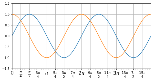

import datetime 
import numpy as np
import matplotlib.pyplot as plt
# Prepare data
x = np.arange(0,10,0.01)
y = np.sin(x)
# Convert data to a list of datetime objects
date_list = []
date_start = datetime.datetime(2000,1,1,0,0,0)
delta = datetime.timedelta(days=1)
for i in range(len(x)):
    date_list.append(date_start + i*delta)
# Drawing, date_list as x-axis data is passed as a parameter
fig, ax = plt.subplots(figsize=(10,4))
plt.plot(date_list, y)
# Set title
plt.title('datetime example')
plt.ylabel('data')
plt.xlabel('Date')
plt.show()
plt.close()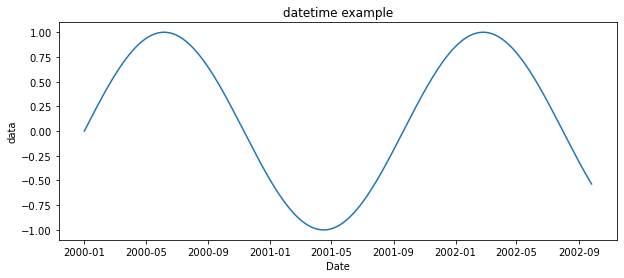

If there is time and date information in the data, you can use strptime and strftime to convert directly.

Use the strptime function to convert a string to time, and use strftime to convert time to a string.

Time and date formatting symbols in python:

Symbol	significance
%y	Two digit year representation (00-99)
%Y	Four digit year representation (000-9999)
%m	Month (01-12)
%d	Day of the month (0-31)
%H	24-hour system hours (0-23)
%I	12 hour system hours (01-12)
%M	Minutes (00 = 59)
%S	Seconds (00-59)
%a	Local simplified week name
%A	Local full week name
%b	Local simplified month name
%B	Local full month name
%c	Local corresponding date representation and time representation
%j	Day of the year (001-366)
%p	Equivalent of local A.M. or P.M
%U	Number of weeks in a year (00-53) Sunday is the beginning of the week
%w	Week (0-6), Sunday is the beginning of the week
%W	Number of weeks in a year (00-53) Monday is the beginning of the week
%x	Local corresponding date representation
%X	Local corresponding time representation
%Z	The name of the current time zone
%%	%Number itself

Keywords: Python MATLAB Back-end

Added by stevehossy on Mon, 22 Nov 2021 04:36:49 +0200

Programming VIP