catalogue

preface

1, Mission

2, Implementation and analysis

1. Import and storage

2. Construct data model

3. Render map elements

 4. Perform the query operation and complete the drawing

3, Summary

preface

This book assumes that readers understand the basic knowledge of Pyhon and information technology, and at least have a certain understanding of geospatial analysis.

It describes the code implementation and analysis of the "big test" part of Python and geospatial analysis in Chapter 1.

1, Mission

Now that you have a better understanding of geospatial analysis, let's start building a name using Python
For the GIS application of SimpleGIS. This program will build a complete GIS application using geographic data model, and can
Render a thematic map showing the population of different cities.
The data model will also be structured, so you can do some basic query operations. SimpleGIS will include Corot
Three cities in Lado state and their population.
More importantly, we will build this small system entirely using Python code to demonstrate the python language
The power of words. Of course, we will also use some modules in the Python standard library, but we will not download any third-party application packages.

The Python version used by the author is 3.9, and the IDE is VScode. Other ides can refer to this: Recommend 10 best Python IDE rookie tutorials (runoob.com)

2, Implementation and analysis

The main analysis of this part is in the comments.

1. Import and storage

The only external library used is turtle, a drawing library commonly used by beginners.

import turtle as t

2. Construct data model

First declare some constants related to all cities.

# In computer science, it is a common practice to put commonly used numbers in variables convenient for memory. This variable is often called a constant.
# The beauty is that indexes can do the same.
# The following three constants actually specify the order of elements in the list, that is, the first is the name, the second is the point coordinate (longitude and latitude), and the third is the population.

NAME = 0
POINTS = 1
POP = 2

# Colorado has 5187582 people with latitude between 37 and 41 degrees north and longitude between 102 and 109 degrees west.
state = ["COLORADO", [[-109, 37],[-109, 41],[-102, 41],[-102,37]], 5187582]

# city
cities = []
cities.append(["DENVER",[-104.98, 39.74], 634265])
cities.append(["BOULDER",[-105.27, 40.02], 98889])
cities.append(["DURANGO",[-107.88,37.28], 17069])

Then define the map size and determine the drawing boundary, and define a conversion function to convert the world coordinates (longitude and latitude) into screen coordinates.

# Map size
map_width = 400
map_height = 300

# First, we need to determine the maximum range, that is, the size of the state.
# First assume a range. Interestingly, the assumed minimum is large, but the maximum is small.
minx = 180
maxx = -180
miny = 90
maxy = -90
# The beauty of this loop is that the boundary value can be determined even if the map boundary to be drawn is not square.
# In fact, the minimum circumscribed rectangle (MBR) is determined.
for x,y in state[POINTS]:
    if x < minx: minx = x
    elif x > maxx: maxx = x
    if y < miny: miny = y
    elif y > maxy: maxy = y
# Step 2 is to calculate the scaling between the state and the drawing board This scale is used to convert longitude and latitude coordinates into screen coordinates.
# We obtain the size of the state in x and y coordinates, and then compare it with the size of the map to obtain the scaling scale:
dist_x = maxx - minx
dist_y = maxy - miny
x_ratio = map_width / dist_x
y_ratio = map_height / dist_y

# Conversion function
def convert(point):
    # lon: longitude lat: Dimension
    lon = point[0]
    lat = point[1]
    x = map_width - ((maxx - lon) * x_ratio)
    y = map_height - ((maxy - lat) * y_ratio)
    # The center of the screen is the starting point of the turtle graphics engine, so the position of the coordinate points must be offset appropriately
    x = x - (map_width/2)
    y = y - (map_height/2)
    return [x,y]

The detailed description is shown in the figure:

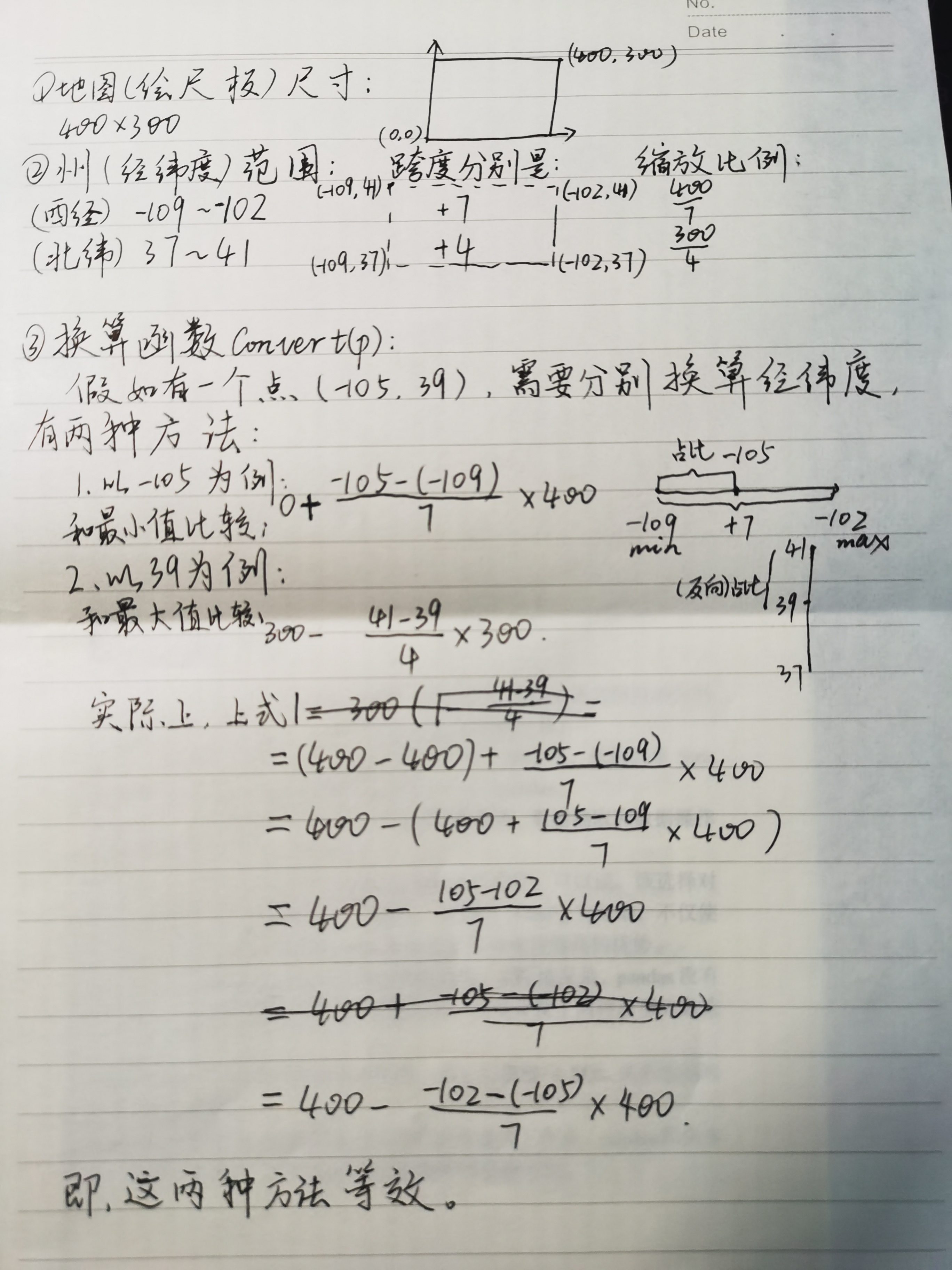
Description of the convert function

3. Render map elements

First draw the boundary.

# Start drawing
t.up()
# The purpose of setting variables for the first position is to draw a closed figure without adding a point to the coordinate list.
first_pixel = None
for point in state[POINTS]:
    pixel = convert(point)
    if not first_pixel:
        first_pixel = pixel
    t.goto(pixel)
    t.down()
t.goto(first_pixel)
t.up()
t.goto([0,0])
t.write(state[NAME], align="center", font=("Arial",16,"bold"))

Then draw the city. Note that the method of using the convert function here is different from the above, showing the author's ingenious idea when defining the function.

# Draw City
for city in cities:
    pixel = convert(city[POINTS])
    t.up()
    t.goto(pixel)
    # Draw City Location
    t.dot(10)
    # Mark city
    t.write(city[NAME] + ", Pop.: " + str(city[POP]), align="left")
    t.up()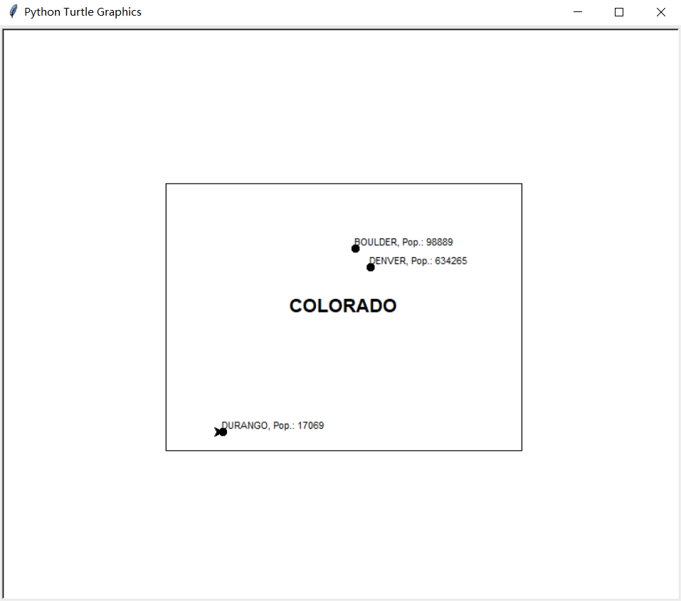

Renderings

 4. Perform the query operation and complete the drawing

# Perform an attribute query operation to determine the most populous city
biggest_city = max(cities, key=lambda city:city[POP])
t.goto(0,-200)
t.write("The biggest city is: " + biggest_city[NAME])
# Perform an attribute query operation to determine the westernmost city
western_city = min(cities, key=lambda city:city[POINTS])
t.goto(0,-220)
t.write("The western-most city is: " + western_city[NAME])
# Close brush
t.pen(shown=False)
# Use t.done() to save the form
t.done()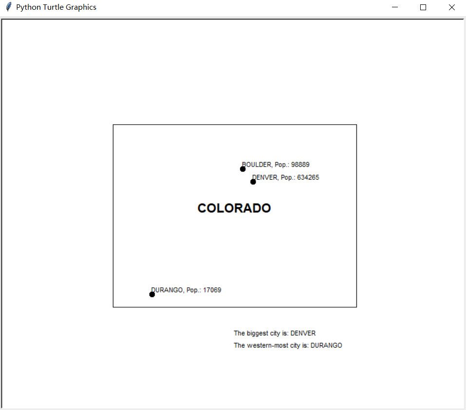

design sketch

3, Summary

This paper briefly introduces the code implementation of the "ox knife test". In fact, the mathematical principle is also very simple. You can deduce the coordinate conversion formula without advanced mathematics. You can draw and combine the graphics to deepen your understanding.