We will build a logistic regression model to predict whether a student is admitted to the University. Suppose you are an administrator of a university department. You want to decide the admission opportunity of each applicant according to the results of two exams. You have the historical data of previous applicants, and you can use it as the training set of logistic regression.
Here we have a LogiReg_data.txt file data:

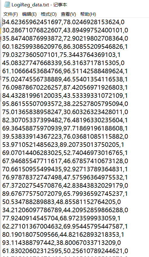
For each training example, you have two exam applicants' scores and admission decisions. In order to do this, we will establish a classification model to estimate the enrollment probability according to the examination results.

First import three major pieces of data analysis:

import numpy as np
import pandas as pd
import matplotlib.pyplot as plt
%matplotlib inline

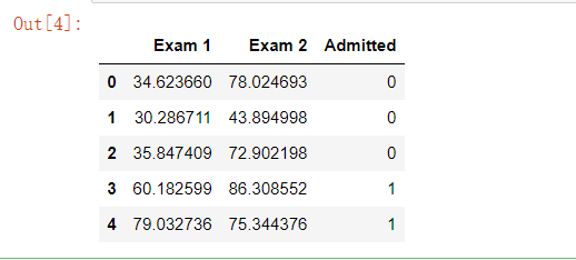
Import the data and set the header, 'Exam 1', and 'Exam 2', indicating the scores of two subjects, 'accepted' indicating whether to be Admitted. Read the first five data in the form to see the effect:

import os
path = 'data' + os.sep + 'LogiReg_data.txt'
pdData = pd.read_csv(path, header=None, names=['Exam 1', 'Exam 2', 'Admitted'])
pdData.head()

Take a look at the scale of our data:

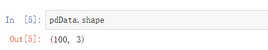
It can be seen that there are 100 pieces of data with 3 columns of characteristics.

We can plot to see the distribution of 0 or 1 on the image:

positive = pdData[pdData['Admitted'] == 1]
negative = pdData[pdData['Admitted'] == 0] 

fig, ax = plt.subplots(figsize=(10,5))
ax.scatter(positive['Exam 1'], positive['Exam 2'], s=30, c='b', marker='o', label='Admitted')
ax.scatter(negative['Exam 1'], negative['Exam 2'], s=30, c='r', marker='x', label='Not Admitted')
ax.legend()
ax.set_xlabel('Exam 1 Score')
ax.set_ylabel('Exam 2 Score')

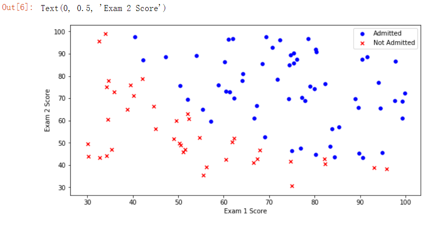
We can clearly see the general distribution of admission and non admission. For these two distributions, we should try to draw a decision boundary to separate the two types. Next, we begin to use the logistic regression algorithm.

First of all, we should clarify our goal: establish a classifier (solve the three parameters 𝜃 0, 𝜃 1 and 𝜃 2, and the distribution represents the three eigenvalues of 'Exam 1', 'Exam 2' and 'accepted'), and then consider setting the threshold to judge the admission result according to the threshold. We generally use 0.5 here, if it is greater than 0.5, we will be Admitted, and if it is less than 0.5, we will not be Admitted.

Modules to be completed:

• sigmoid: function mapped to probability

• model: returns the prediction result value

• cost: calculate the loss according to the parameters

• Gradient: calculate the gradient direction of each parameter

• descent: update parameters

• Accuracy: calculation accuracy

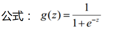
1. Function sigmoid mapped to probability

Code implementation:

def sigmoid(z):
    return 1 / (1 + np.exp(-z))

Remember what it looks like? Let's draw:

nums = np.arange(-10, 10, step=1) 
fig, ax = plt.subplots(figsize=(12,4))
ax.plot(nums, sigmoid(nums), 'r')

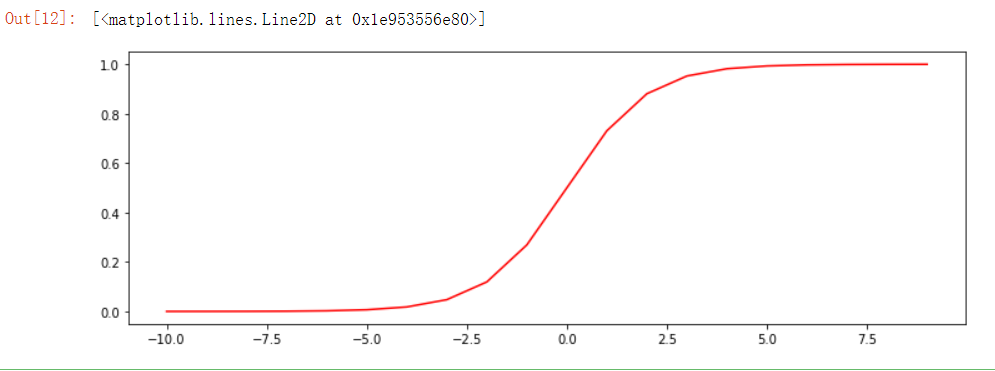
It is obvious that:
𝑔:ℝ→[0,1]
𝑔(0)=0.5
𝑔(−∞)=0
𝑔(+∞)=1

2. Return prediction result value model function

Next, we complete the prediction function model,

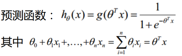
Here we are:

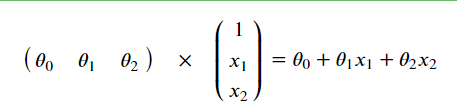
Why is x1,x2 above 1? Remember when we were Principle derivation of linear regression algorithm
It is mentioned in that during numerical calculation, in order to make the whole be expressed in the form of matrix, even if there is no x0 item, it can be added manually. Just add a column of x0 in the data and make its values all 1, and the result remains unchanged.

model function code implementation:

def model(X, theta):
    
    return sigmoid(np.dot(X, theta.T))

next

pdData.insert(0, 'Ones', 1) # Add a new column with all 1 values, and specify Ones for the column name

orig_data = pdData.values # Convert DataFrame to array
cols = orig_data.shape[1]
X = orig_data[:,0:cols-1]
y = orig_data[:,cols-1:cols]

#Construct theta occupation, usually filled with 0, 1 row and 3 columns
theta = np.zeros([1, 3])

Let's see if there is any problem with the data:

We can see that there is no problem with the data, which is in line with our expectations.

3. Calculate the loss value cost

Here, the data is ready. Next, we will calculate the loss according to the parameters. First, define the loss function:

Loss function code:

def cost(X, y, theta):
    left = np.multiply(-y, np.log(model(X, theta)))
    right = np.multiply(1 - y, np.log(1 - model(X, theta)))
    return np.sum(left - right) / (len(X))

After writing the loss function, let's call it to see the loss value:

Now we don't care whether the loss value is large or small, as long as we know that we can calculate it and the formula is easy to use 🆗 Yes.

4. Calculate gradient

Then we should calculate the gradient. Before, we spent a lot of effort in logical regression to find the partial derivative:

Write the gradient calculation function accordingly:

def gradient(X, y, theta):
    grad = np.zeros(theta.shape)
    error = (model(X, theta)- y).ravel()
    for j in range(len(theta.ravel())): 
        term = np.multiply(error, X[:,j])
        grad[0, j] = np.sum(term) / len(X)
    
    return grad

According to the number of iterations, loss value and gradient, we can get three different gradient descent methods:

STOP_ITER = 0
STOP_COST = 1
STOP_GRAD = 2

def stopCriterion(type, value, threshold):
    #Set three different stop strategies
    if type == STOP_ITER:        return value > threshold
    elif type == STOP_COST:      return abs(value[-1]-value[-2]) < threshold
    elif type == STOP_GRAD:      return np.linalg.norm(value) < threshold

5. Update parameters

When we update iteratively, in order to generalize the model, we will try to disrupt the data, that is, shuffle:

import numpy.random
#shuffle the cards
def shuffleData(data):
    np.random.shuffle(data)
    cols = data.shape[1]
    X = data[:, 0:cols-1]
    y = data[:, cols-1:]
    return X, y

Then solve the gradient descent:

import time

def descent(data, theta, batchSize, stopType, thresh, alpha):
    #Gradient descent solution
    
    init_time = time.time()
    i = 0 # Number of iterations
    k = 0 # batch
    X, y = shuffleData(data)
    grad = np.zeros(theta.shape) # Calculated gradient
    costs = [cost(X, y, theta)] # magnitude of the loss

    
    while True:
        grad = gradient(X[k:k+batchSize], y[k:k+batchSize], theta)
        k += batchSize #Take batch quantity data
        if k >= n: 
            k = 0 
            X, y = shuffleData(data) #Reshuffle
        theta = theta - alpha*grad # Parameter update
        costs.append(cost(X, y, theta)) # Calculate new losses
        i += 1 

        if stopType == STOP_ITER:       value = i
        elif stopType == STOP_COST:     value = costs
        elif stopType == STOP_GRAD:     value = grad
        if stopCriterion(stopType, value, thresh): break
    
    return theta, i-1, costs, grad, time.time() - init_time

Write another drawing function:

def runExpe(data, theta, batchSize, stopType, thresh, alpha):
    theta, iter, costs, grad, dur = descent(data, theta, batchSize, stopType, thresh, alpha)
    name = "Original" if (data[:,1]>2).sum() > 1 else "Scaled"
    name += " data - learning rate: {} - ".format(alpha)
    if batchSize==n: strDescType = "Gradient"
    elif batchSize==1:  strDescType = "Stochastic"
    else: strDescType = "Mini-batch ({})".format(batchSize)
    name += strDescType + " descent - Stop: "
    if stopType == STOP_ITER: strStop = "{} iterations".format(thresh)
    elif stopType == STOP_COST: strStop = "costs change < {}".format(thresh)
    else: strStop = "gradient norm < {}".format(thresh)
    name += strStop
    print ("***{}\nTheta: {} - Iter: {} - Last cost: {:03.2f} - Duration: {:03.2f}s".format(
        name, theta, iter, costs[-1], dur))
    fig, ax = plt.subplots(figsize=(12,4))
    ax.plot(np.arange(len(costs)), costs, 'r')
    ax.set_xlabel('Iterations')
    ax.set_ylabel('Cost')
    ax.set_title(name.upper() + ' - Error vs. Iteration')
    return theta

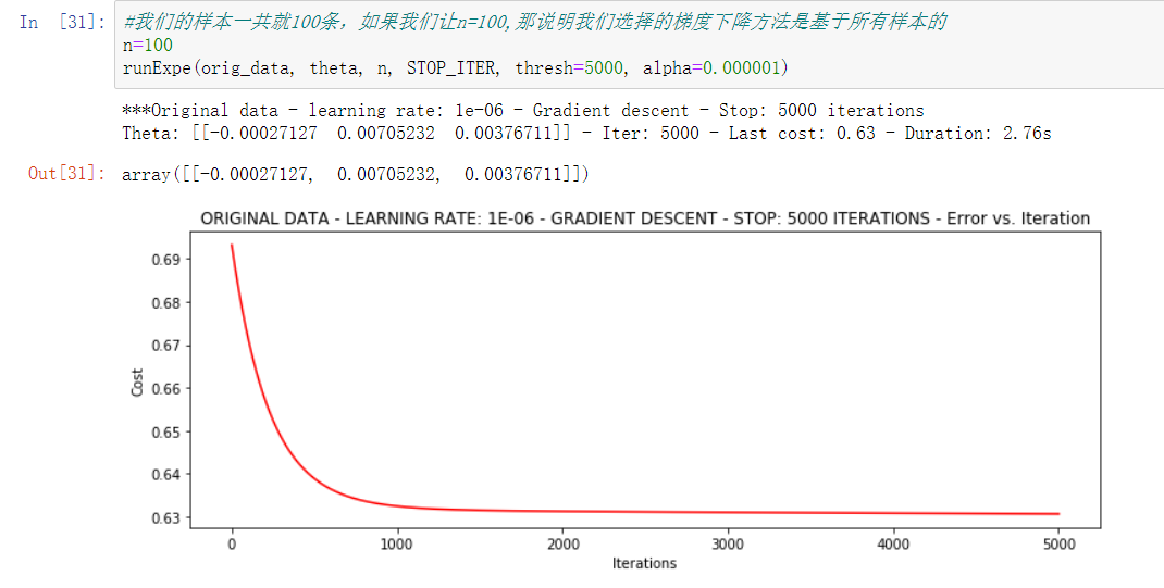
1. Based on the number of iterations to stop

#We have a total of 100 samples. If we let n=100, it means that the gradient descent method we choose is based on all samples
n=100
runExpe(orig_data, theta, n, STOP_ITER, thresh=5000, alpha=0.000001) # 5000 iterations

2. Stop according to the loss value

Setting the threshold 1E-6 requires almost 110000 iterations,

runExpe(orig_data, theta, n, STOP_COST, thresh=0.000001, alpha=0.001)

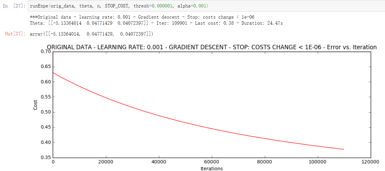
The previous strategy converges to about 0.63 after 5000 iterations, and this time it converges to 0.35-0.40 according to the loss value stop strategy method. It can be seen that this iterative strategy is better than the previous one.

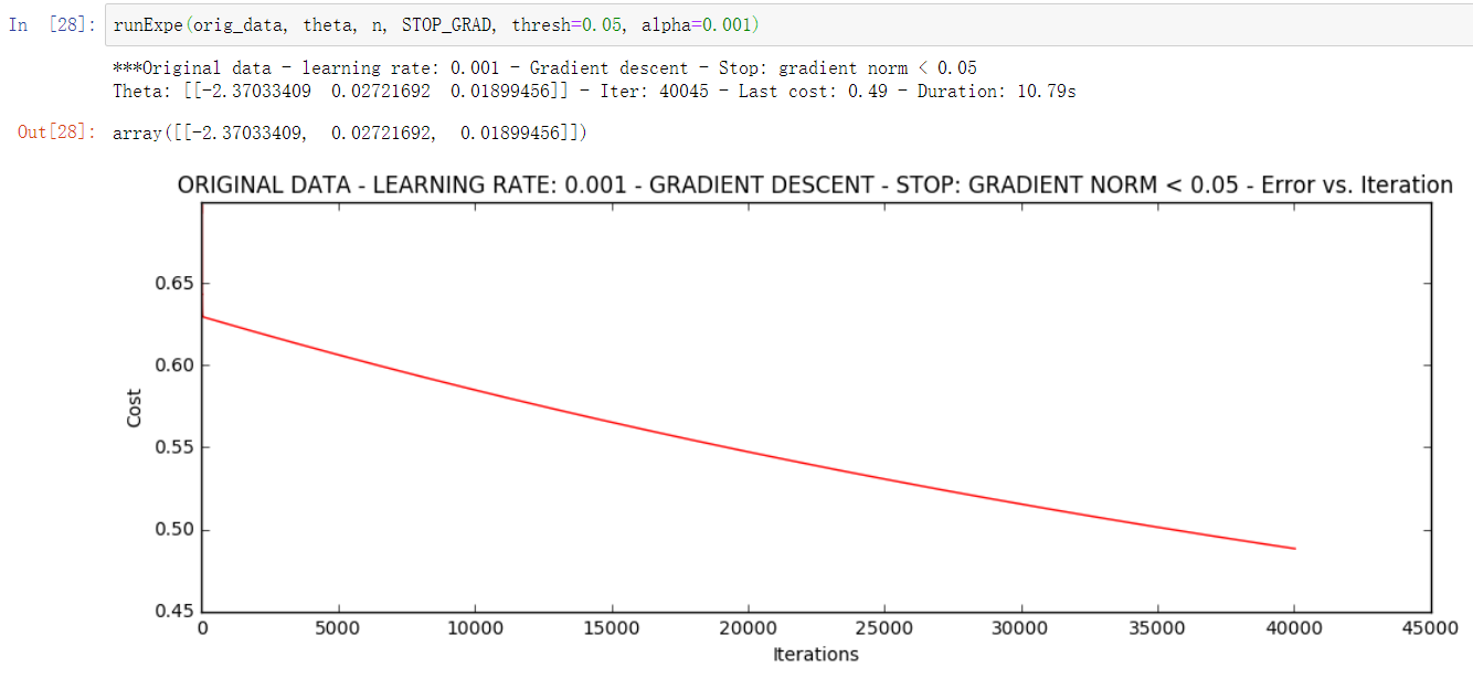
1. Stop according to gradient change
   Setting a threshold of 0.05 requires almost 40000 iterations.

runExpe(orig_data, theta, n, STOP_GRAD, thresh=0.05, alpha=0.001)

The above three kinds of strategies we compare are stop strategies. Below we compare different gradient descent methods:

• Random gradient descent

runExpe(orig_data, theta, 1, STOP_ITER, thresh=5000, alpha=0.001) # One sample per iteration

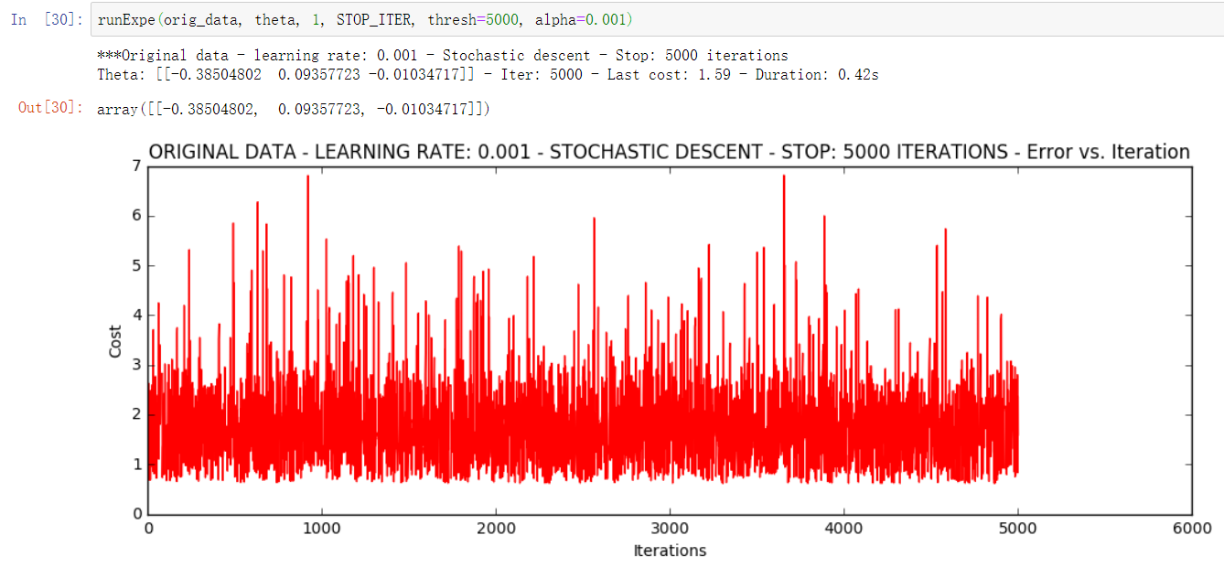
It looks very unstable. Let's try to reduce the learning rate:

runExpe(orig_data, theta, 1, STOP_ITER, thresh=15000, alpha=0.000002)

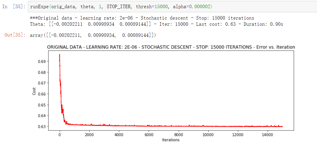
It can be seen that the speed is fast, but the stability is poor, and a small learning rate is required.

• Mini batch descent

runExpe(orig_data, theta, 16, STOP_ITER, thresh=15000, alpha=0.001)

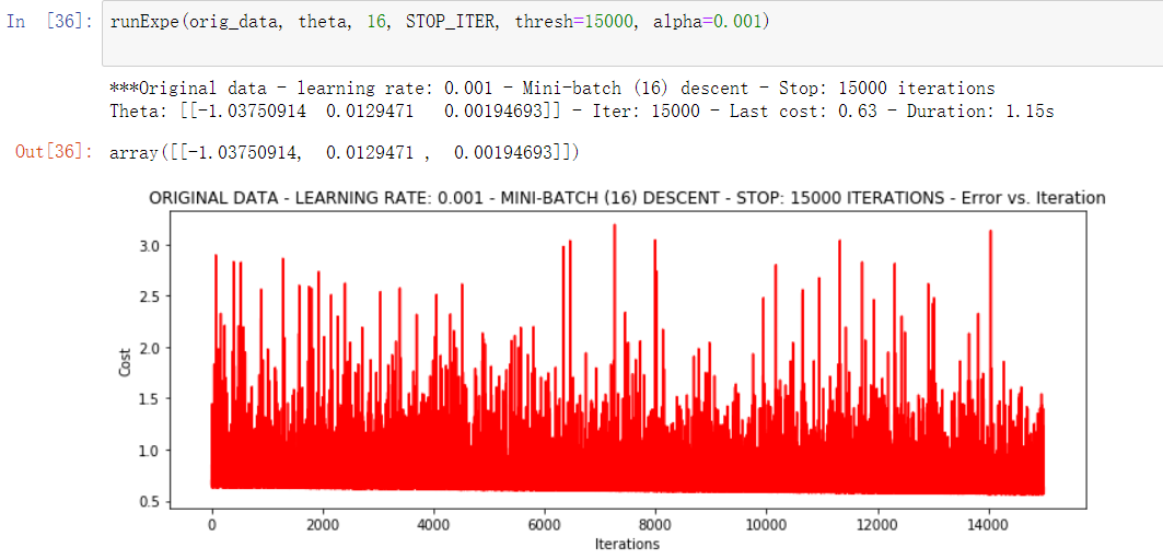
The fluctuation is still relatively large. We will not adjust the learning rate this time. In another way, let's try to standardize the data, subtract its mean value according to its attribute (by column), and then divide it by its variance. The final result is that for each attribute / column, all data are clustered around 0, and the variance value is 1:

from sklearn import preprocessing as pp

scaled_data = orig_data.copy()
scaled_data[:, 1:3] = pp.scale(orig_data[:, 1:3])

runExpe(scaled_data, theta, n, STOP_ITER, thresh=5000, alpha=0.001)

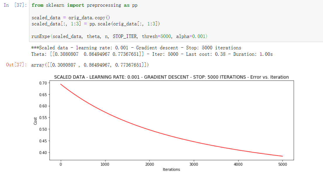
This is much better. The original data can only reach 0.63, while we reach 0.38 here! Therefore, it is very important to preprocess the data.

runExpe(scaled_data, theta, n, STOP_GRAD, thresh=0.02, alpha=0.001)

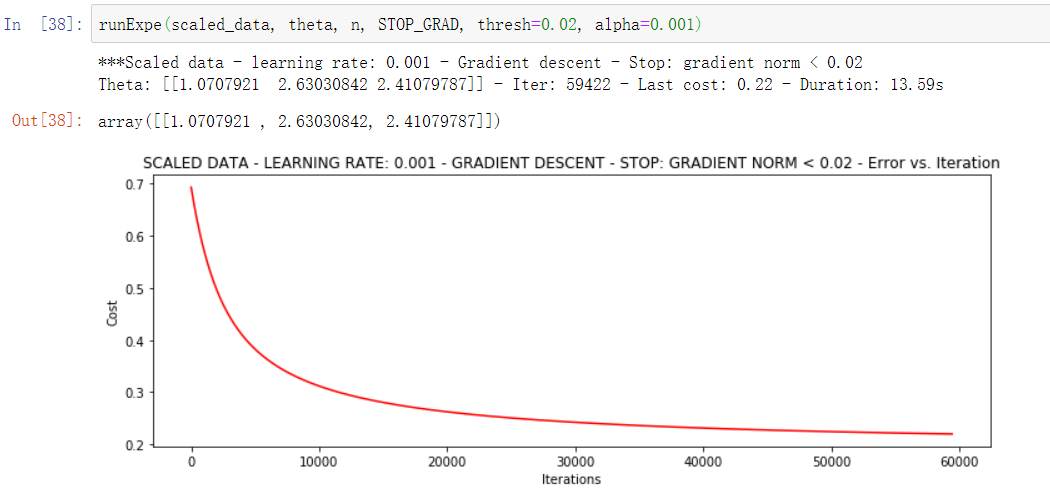
More iterations will reduce the loss more!

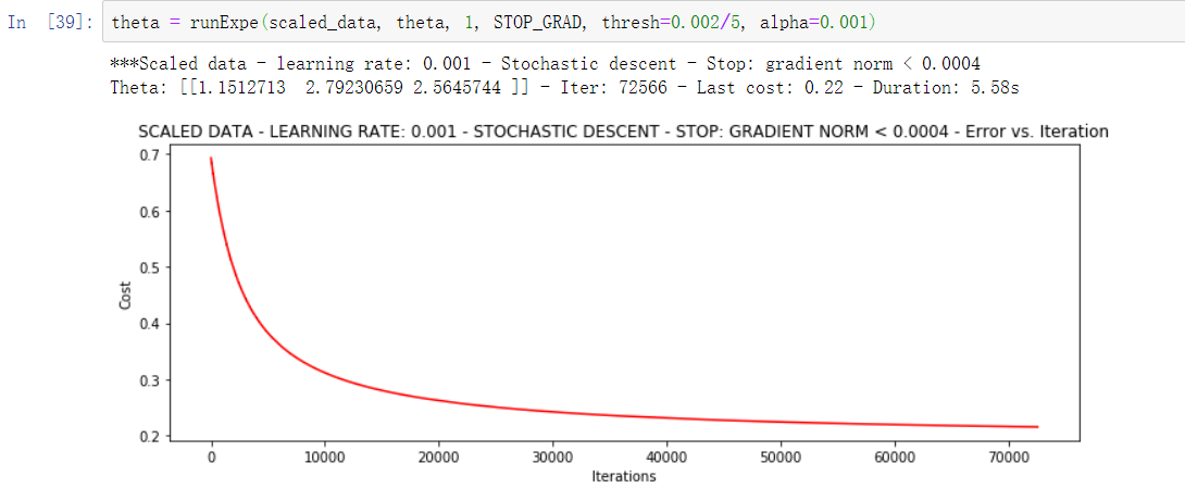
theta = runExpe(scaled_data, theta, 1, STOP_GRAD, thresh=0.002/5, alpha=0.001)

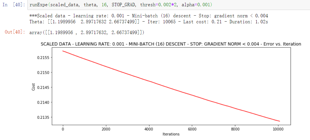
The random gradient drops faster, but we need more iterations, so it's better to use batch!!!

runExpe(scaled_data, theta, 16, STOP_GRAD, thresh=0.002*2, alpha=0.001)

6. Calculation accuracy

Finally, let's calculate the accuracy. First, if the predicted value is greater than 0.5, we will be admitted. Otherwise, we will not be admitted,

#Set threshold
def predict(X, theta):
    return [1 if x >= 0.5 else 0 for x in model(X, theta)]

Calculation accuracy:

scaled_X = scaled_data[:, :3]
y = scaled_data[:, 3]
predictions = predict(scaled_X, theta)
correct = [1 if ((a == 1 and b == 1) or (a == 0 and b == 0)) else 0 for (a, b) in zip(predictions, y)]
accuracy = (sum(map(int, correct)) % len(correct))
print ('accuracy = {0}%'.format(accuracy))

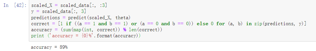
Through our gradient descent and logistic regression algorithm, we calculate that the accuracy is 89%.

Summary:

Two core algorithms in machine learning: linear regression and logical regression are applied to regression and classification tasks respectively. In the process of solving, the core idea of machine learning is to optimize the solution and constantly find the most appropriate parameters, which leads to the gradient descent algorithm. In the actual training model, we also need to consider the impact of various parameters on the results. In subsequent practical cases, these need to be adjusted through experiments. In the process of principle derivation, many small knowledge points are involved, which are not unique to a certain algorithm. Their shadow will be seen in the subsequent algorithm learning process. Slowly, you will find various routines in machine learning.