What is stock selection?
Stock selection is an active investment strategy. First, analyze the prospect of a single stock according to some rules or algorithms, and then build a portfolio for long-term holding. Generally, the stocks of the portfolio are required to have low correlation, so as to hedge the systemic risk. Otherwise, when the market weakens, the portfolio will also face huge downside risk.
What model is used?
On how to select stocks, academia has put forward many different models, and the most classic is Markowitz's portfolio theory. Here, we use the MM trend template, which is a technical stock selection method proposed by a legendary foreign investment master. The core idea is to measure the stock kinetic energy through technical indicators, select the most potential stocks, buy and hold them.
MM trend model
- The stock price is higher than the 150 day moving average and the 200 day moving average
- The 150 day moving average is higher than the 200 day moving average
- The 200 day moving average rose for at least one month
- The 50 day moving average is higher than the 150 day moving average and the 200 day moving average
- The stock price is higher than the 50 day moving average
- The stock price is 30% higher than the 52 week low
- The stock price is within 25% of the 52 week high
- The relative strength index (RS) is greater than or equal to 70. Here, the relative strength refers to the comparison between the stock and the market. Rs = 1-year return of the stock / 1-year return of the benchmark index
About Mark Minervini
One of the most famous traders in the United States, who once earned a yield of 30000%, was called a billionaire before the age of 34. See the book "financial geek" for details.
Technical problems faced by stock selection?
- Where can I get a lot of historical data of stocks?
- How to improve computing performance when there are a large number of stocks?
This paper will use Python to realize the quantitative stock selection of MM model, and solve the above two technical problems.
import os
import datetime as dt
import time
from typing import Any, Dict, Optional, List

import requests
import pickle
import numpy as np
import pandas as pd
import matplotlib.pyplot as plt
import seaborn as sns
import talib
import multiprocessing as mp
from requests.exceptions import ConnectionError, Timeout

%matplotlib inline
plt.style.use("fivethirtyeight")
1. Obtain historical data from hummingbird data
Hummingbird data It is an emerging financial data provider, providing real-time quotation and historical data including stocks, foreign exchange, commodity futures and digital currency, and providing API interface , it is a convenient channel for all financial practitioners to obtain free data.
## Write custom functions and obtain data through API

def fetch_trochil(url: str,
                  params: Dict[str, str],
                  attempt: int = 3,
                  timeout: int = 3) -> Dict[str, Any]:
    """decorate requests.get function"""
    for i in range(attempt):
        try:
            resp = requests.get(url, params, timeout=timeout)
            resp.raise_for_status()
            data = resp.json()["data"]
            if not data:
                raise Exception("empty dataset")
            return data
        except (ConnectionError, Timeout) as e:
            print(e)
            i += 1
            time.sleep(i * 0.5)


def fetch_cnstocks(apikey: str) -> pd.DataFrame:
    """Get from hummingbird data A Stock product list"""
    url = "https://api.trochil.cn/v1/cnstock/markets"
    params = {"apikey": apikey}

    res = fetch_trochil(url, params)

    return pd.DataFrame.from_records(res)


def fetch_daily_ohlc(symbol: str,
                     date_from: dt.datetime,
                     date_to: dt.datetime,
                     apikey: str) -> pd.DataFrame:
    """Get from hummingbird data A Stock day chart history K Line"""
    url = "https://api.trochil.cn/v1/cnstock/history"
    params = {
        "symbol": symbol,
        "start_date": date_from.strftime("%Y-%m-%d"),
        "end_date": date_to.strftime("%Y-%m-%d"),
        "freq": "daily",
        "apikey": apikey
    }

    res = fetch_trochil(url, params)

    return pd.DataFrame.from_records(res)


def fetch_index_ohlc(symbol: str,
                     date_from: dt.datetime,
                     date_to: dt.datetime,
                     apikey: str) -> pd.DataFrame:
    """Obtain the daily chart historical data of the stock index"""
    url = "https://api.trochil.cn/v1/index/daily"
    params = {
        "symbol": symbol,
        "start_date": date_from.strftime("%Y-%m-%d"),
        "end_date": date_to.strftime("%Y-%m-%d"),
        "apikey": apikey
    }

    res = fetch_trochil(url, params)

    return pd.DataFrame.from_records(res)
1.1 product list
First obtain all stock ID s of Shanghai and Shenzhen A-share listed enterprises.
apikey = os.getenv("TROCHIL_API")  # use your apikey
cnstocks = fetch_cnstocks(apikey)
cnstocks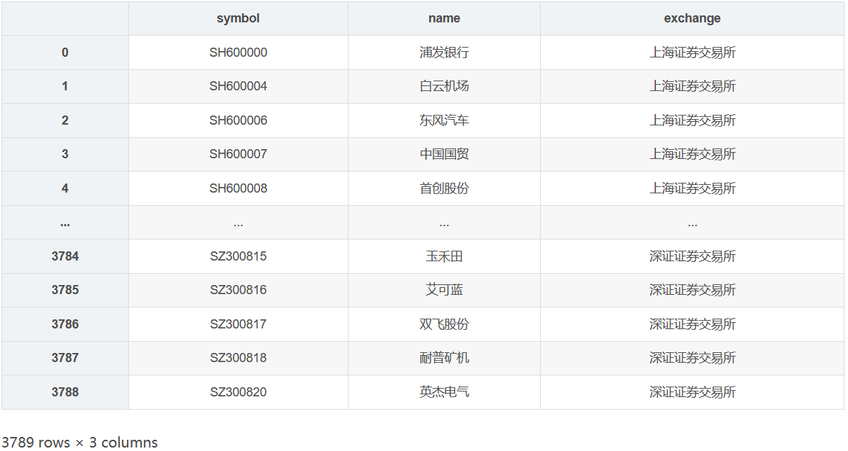
Successfully obtained the product information of 3789 stocks of Shanghai and Shenzhen A shares. The prefix 'SH' represents the stocks of Shanghai Stock Exchange and 'SZ' represents the stocks of Shenzhen Stock Exchange. Only the stocks of Shanghai Stock Exchange are used in modeling.
# Filter stocks prefixed with 'SH'
cnstocks_shsz = cnstocks.query("symbol.str.startswith('SH')")
cnstocks_shsz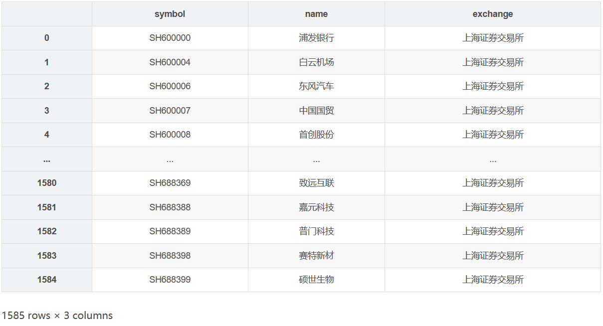
1.2 historical data of individual stocks
Obtain the daily chart historical price of stocks in Shanghai Stock Exchange from hummingbird data. According to the MM trend model, we need at least the historical data of the past 260 days. Some newly listed or delisted stocks may not meet the requirements, so we exclude the stocks with less than 260 K-line.
%%time

# Download historical data from 2019 to the present
# Stocks with K-line less than 260 trading days shall be excluded during downloading
date_from = dt.datetime(2019, 1, 1)
date_to = dt.datetime.today()
symbols = cnstocks_shsz.symbol.to_list()
min_klines = 260

# Download one by one. The API of hummingbird data has no minute request limit
# First store the data in the list, and then merge and clean it after downloading
ohlc_list = []
for symbol in symbols:
    try:
        ohlc = fetch_daily_ohlc(symbol, date_from, date_to, apikey)
        if ohlc is not None and len(ohlc) >= min_klines:
            ohlc.set_index("datetime", inplace=True)
            ohlc_list.append(ohlc)
    except Exception as e:
        pass


CPU times: user 21.7 s, sys: 349 ms, total: 22 s
Wall time: 49.3 s
It takes less than a minute to download the historical data of more than 1500 stocks (about 400 trading days). Next, we integrate and clean the data, and then store it locally for subsequent analysis.
ohlc_joined = pd.concat(ohlc_list)
ohlc_joined.info()


<class 'pandas.core.frame.DataFrame'>
Index: 532756 entries, 2019-01-02 to 2020-07-29
Data columns (total 6 columns):
 #   Column  Non-Null Count   Dtype
---  ------  --------------   -----
 0   open    532756 non-null  float64
 1   high    532756 non-null  float64
 2   low     532756 non-null  float64
 3   close   532756 non-null  float64
 4   volume  532756 non-null  float64
 5   symbol  532756 non-null  object
dtypes: float64(5), object(1)
memory usage: 28.5+ MB
Check for missing values.
ohlc_joined.isnull().sum()


open      0
high      0
low       0
close     0
volume    0
symbol    0
dtype: int64
Save locally and store in csv format. Later, you can read data directly from the local to avoid the waste of time caused by API requests.
ohlc_joined.to_csv("cnstock_daily_ohlc.csv", index=True)1.3 Shanghai Stock Index
Obtain the historical price of Shanghai stock index and calculate the cumulative rate of return in the past year, which is used to calculate the relative strength of individual stocks.
benchmark = fetch_index_ohlc("shci", date_from, date_to, apikey)
benchmark.tail()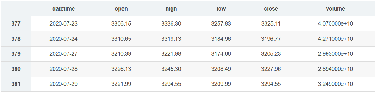
# Calculate the 1-year cumulative rate of return, which is calculated by 252 trading days in 1 year
benchmark_ann_ret = benchmark.close.pct_change(252).iloc[-1]
benchmark_ann_ret


0.12150312157460808
2. Stock selection
def screen(close: pd.Series, benchmark_ann_ret: float) -> pd.Series:
    """realization MM The logic of stock selection model to evaluate whether a single stock meets the screening conditions

    Args:
        close(pd.Series): Stock closing price, default time series index
        benchmark_ann_ret(float): The 1-year yield of the benchmark index is used to calculate the relative strength
    """
    # Calculate the daily moving average of 50150200
    ema_50 = talib.EMA(close, 50).iloc[-1]
    ema_150 = talib.EMA(close, 150).iloc[-1]
    ema_200 = talib.EMA(close, 200).iloc[-1]

    # The 20 day movement of the 200 day moving average is smooth, which is used to judge whether the 200 day moving average rises
    ema_200_smooth = talib.EMA(talib.EMA(close, 200), 20).iloc[-1]

    # 52 week high and 52 week low of closing price
    high_52week = close.rolling(52 * 5).max().iloc[-1]
    low_52week = close.rolling(52 * 5).min().iloc[-1]

    # Latest closing price
    cl = close.iloc[-1]

    # Screening condition 1: the closing price is higher than the 150 day moving average and the 200 day moving average
    if cl > ema_150 and cl > ema_200:
        condition_1 = True
    else:
        condition_1 = False

    # Screening condition 2: the 150 day moving average is higher than the 200 day moving average
    if ema_150 > ema_200:
        condition_2 = True
    else:
        condition_2 = False

    # Screening condition 3: the daily average of 200 rises by 1 month
    if ema_200 > ema_200_smooth:
        condition_3 = True
    else:
        condition_3 = False

    # Screening condition 4: the 50 day moving average is higher than the 150 day moving average and the 200 day moving average
    if ema_50 > ema_150 and ema_50 > ema_200:
        condition_4 = True
    else:
        condition_4 = False

    # Screening condition 5: the closing price is higher than the 50 day moving average
    if cl > ema_50:
        condition_5 = True
    else:
        condition_5 = False

    # Screening condition 6: the closing price is 30% higher than the 52 week low
    if cl >= low_52week * 1.3:
        condition_6 = True
    else:
        condition_6 = False

    # Screening condition 7: the closing price is within 25% of the 52 week high
    if cl >= high_52week * 0.75 and cl <= high_52week * 1.25:
        condition_7 = True
    else:
        condition_7 = False

    # Screening condition 8: the relative strength index is greater than or equal to 70
    rs = close.pct_change(252).iloc[-1] / benchmark_ann_ret * 100
    if rs >= 70:
        condition_8 = True
    else:
        condition_8 = False

    # Judge whether the stock meets the standard
    if (condition_1 and condition_2 and condition_3 and
        condition_4 and condition_5 and condition_6 and
        condition_7 and condition_8):
        meet_criterion = True
    else:
        meet_criterion = False

    out = {
        "rs": round(rs, 2),
        "close": cl,
        "ema_50": ema_50,
        "ema_150": ema_150,
        "ema_200": ema_200,
        "high_52week": high_52week,
        "low_52week": low_52week,
        "meet_criterion": meet_criterion
    }

    return pd.Series(out)
2.1 synchronization
Firstly, we use the synchronous method to filter, and apply the same filter function to 1400 stocks.
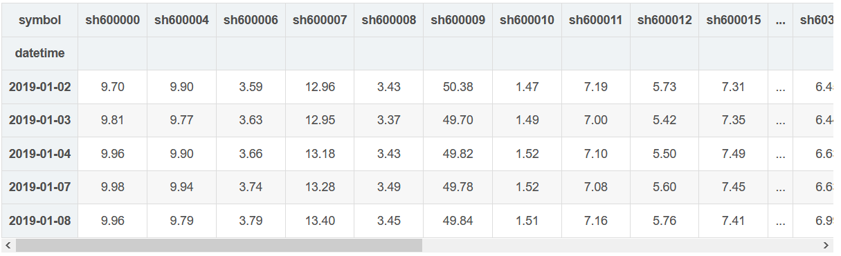
# Only select stocks with sufficient historical data
symbols_to_screen = list(ohlc_joined.symbol.unique())

# Convert the format of data frame from long format to wide format
ohlc_joined_wide = ohlc_joined.pivot(columns="symbol", values="close").fillna(method="ffill")

ohlc_joined_wide.head()
%%time

results = ohlc_joined_wide.apply(screen, benchmark_ann_ret=benchmark_ann_ret)
results = results.T


CPU times: user 2.97 s, sys: 6.47 ms, total: 2.98 s
Wall time: 2.97 s
Synchronous calculation takes about 3 seconds, which is acceptable in the research stage, but not in the production stage. Imagine you make the stock selection system into a product. After the user selects the conditions and clicks the filter, it takes at least 3 seconds to get the results, which will lead to a very bad user experience. Next, we try to solve this problem with multiple processes.
Let's first look at the stocks that meet the conditions?
results.query("meet_criterion == True").sort_values("rs", ascending=False)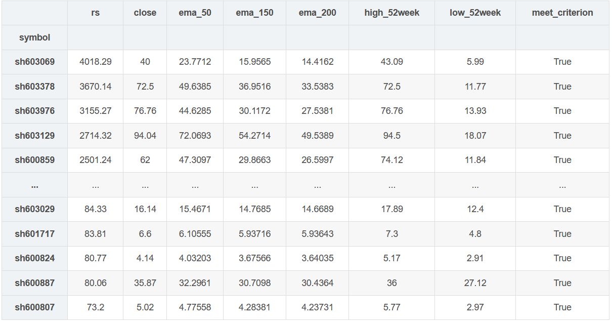
389 stocks are eligible. From the perspective of quantitative trading, it seems that they have not successfully selected potential stocks. Of course, this is related to the selection of parameters.
Whether the model is effective is not the subject of this article (we will explore it in other articles), so don't pay too much attention to this first.
2.2 multi process
Next, try to speed up the stock selection process with multiple processes to see if you can reduce the screening time to less than 1 second. The core idea of multiprocess computing is divide and conquer, distribute similar computing tasks to different CPU s, and finally summarize the results. Here, multiprocessing is used to realize multiprocessing.
%%time

# Define worker function
def screen_stocks(df: pd.DataFrame, benchmark_ann_ret: float) -> pd.DataFrame:
    results = df.apply(screen, benchmark_ann_ret=benchmark_ann_ret)
    return results.T

# To split the data frame, first try to split the data frame into four parts (divided by columns) with four processes
df_chunks = np.array_split(ohlc_joined_wide, 4, axis=1)

# Use multiprocessing The pool object manages the process pool
with mp.Pool(processes=4) as p:
    future_results = [p.apply_async(
        screen_stocks, kwds={"df": df, "benchmark_ann_ret": benchmark_ann_ret}) for df in df_chunks]
    results = pd.concat([r.get() for r in future_results])


CPU times: user 934 ms, sys: 204 ms, total: 1.14 s
Wall time: 1.06 s
Using four processes, we successfully shorten the calculation time to about 1 second, and get the same results.
results.query("meet_criterion == True").sort_values("rs", ascending=False)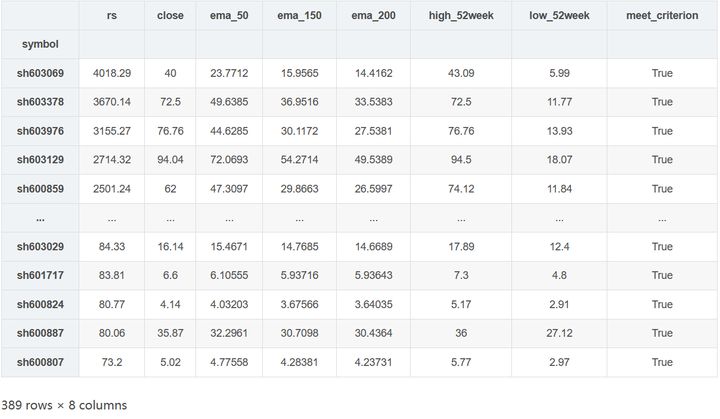
Next, test the relationship between the number of processes and the calculation time to determine the optimal number of processes.
max_processors = mp.cpu_count()

time_used = {}
for processors in range(1, max_processors + 1):
    df_chunks = np.array_split(ohlc_joined_wide, processors, axis=1)
    t0 = time.time()
    with mp.Pool(processors) as p:
        future_results = [p.apply_async(
            screen_stocks, kwds={"df": df, "benchmark_ann_ret": benchmark_ann_ret}) for df in df_chunks]
        results = pd.concat([r.get() for r in future_results])
    elapsed = time.time() - t0
    time_used[processors] = elapsed

fig, ax = plt.subplots(figsize=(12, 7))
ax = sns.pointplot(x=list(time_used.keys()), y=list(time_used.values()))
ax.set_xlabel("CPU cores")
ax.set_ylabel("Time used(seconds)")
ax.set_title("Computation time vs CPU Cores", loc="left")
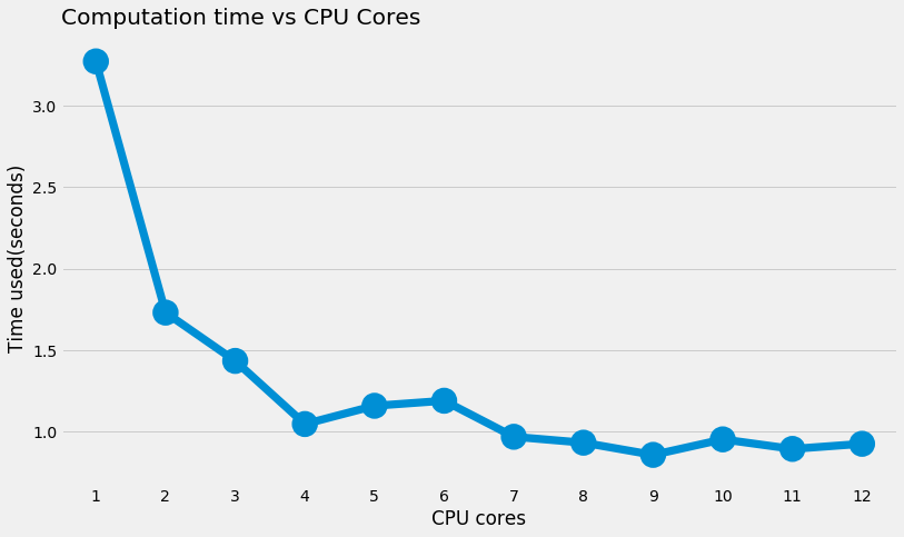
As can be seen from the figure above, the calculation time is reduced by half when using two processes (as expected). As the number of processes approaches the maximum number of processes, the decrease of computing time continues to decline, which is not difficult to understand. Because the computer is processing other tasks at the same time, it is impossible to make full use of all processes even if processors=12 is set. From the current situation, it is appropriate to use four processes to process, which can reduce the time from 3.5 seconds to about 1 second.
3. Summary
This article describes how to use Python for quantitative stock selection, including:
- Obtain the historical data of Shanghai and Shenzhen A shares from hummingbird data.
- User defined functions realize the stock selection logic of MM model.
- Multi process computing greatly reduces the time of filtering.
The next research direction is backtracking test. Build the portfolio according to MM model and optimize the screening parameters to see whether it can bring excess returns.
If you like our articles, remember to praise and collect them. We will continue to bring you high-quality articles in the field of data science and quantitative trading.
[about us]
Hummingbird data : open source financial database, aggregating 10000 + time series of mainstream financial markets, providing high-quality free data for the majority of financial practitioners. Our advantages: 1 At the same time, provide real-time quotation and historical data of stocks, foreign exchange and commodity futures; 2. Provide a highly unified API interface. You can integrate the data into your own program and view our API documentation.
This is an era of big data. The mission of hummingbird data is to create wealth with data.